challenging problem to discover the adaptive configuration tuning ... In order to apply reinforcement learning to the adaptive configu- ..... same client to reuse it.
Boosting the Performance of Computing Systems through Adaptive Configuration Tuning Haifeng Chen Guofei Jiang Hui Zhang Kenji Yoshihira NEC Laboratories America, 4 Independence Way, Princeton, NJ 08540 Email: {haifeng, gfj, hui, kenji}@nec-labs.com
ABSTRACT Good system performance depends on the correct setting of its configuration parameters. It is observed that such optimal configuration relies on the incoming workload of the system. In this paper, we utilize the Markov decision process(MDP) theory and present a reinforcement learning strategy to discover the complex relationship between the system workload and the corresponding optimal configuration. Considering the limitations of current reinforcement learning algorithms used in system management, we present a different learning architecture to facilitate the configuration tuning task which includes two units: the actor and critic. While the actor realizes a stochastic policy that maps the system state to the corresponding configuration setting, the critic uses a value function to provide the reinforcement feedback to the actor. Both the actor and critic are implemented by multiple layer neural networks, and the error back-propagation algorithm is used to adjust the network weights based on the temporal difference error produced in the learning. Experimental results demonstrate that the proposed learning process can identify the correct configuration tuning rule which in turn improves the system performance significantly.
Categories and Subject Descriptors K.6.4 [Management of Computing and Information Systems]: System Management; I.2.6 [Artificial Intelligence]: Learning
General Terms Algorithms, Management
Keywords system management, reinforcement learning, configuration tuning
1.
INTRODUCTION
The performance of web based computing systems is a critical factor to maximize the revenue of service providers. Although adding newer and faster physical devices to the system may be an alternative to improve the performance, it is sometime more appropriate to properly configure the system so that the performance
Permission to make digital or hard copies of all or part of this work for personal or classroom use is granted without fee provided that copies are not made or distributed for profit or commercial advantage and that copies bear this notice and the full citation on the first page. To copy otherwise, to republish, to post on servers or to redistribute to lists, requires prior specific permission and/or a fee. SAC’09 March 8-12, 2009, Honolulu, Hawaii, U.S.A. Copyright 2009 ACM 978-1-60558-166-8/09/03 ...$5.00.
can be enhanced without any extra cost. A correct configuration setting can fully utilize the system resources and hence lead the system to best quality of services (QoS) such as short request response time and high throughput. There have been a number of black-box optimization methods to search the best configuration of systems offline[12][11][5]. However the offline identified configuration maybe sub-optimal because it is rarely changed during the operation once set in the system. In reality, the system optimal configuration usually depends on the incoming workload. Taking the size of database connection pool in a web based system as an example, while setting a large size of connection pool is good for high workload situations to increase the system throughput, the large pool size is not preferred during low workload due to the extra response time caused by the slow access to the connection table. If we correctly tune the configurations when facing different workloads, the system performance can be further improved. With the increasing complexity of computing systems, however, the relationship between the system workload and its related optimal configuration is usually unknown and highly nonlinear. It is a challenging problem to discover the adaptive configuration tuning rule for performance improvement. While there have been some attempts of using analytical models [1] or feedback control theory [3] to solve the dynamic tuning problem, those methods all relied on certain assumptions such as knowing the workload characteristics or the linear resource usages. It is hard to directly come up with explicit mathematical formula or models to describe system configuration change with respect to the dynamic environment. Due to the incapability of model based methods, the model free approaches have received increasing attentions recently in handling complex system management tasks[8][9]. The reinforcement learning is such a method which learns the management rules in a trialand-error manner through interactions with the system. It is ground in the powerful sequential decision theory, and uses the statistical estimation and maximization technique to identify the best action, i.e. the configuration values, under any system state, i.e. the workload statistics, so that certain reward, i.e. the system performance, can be optimized. Compared with the analytical model and control based approaches, the reinforcement learning can discover arbitrary nonlinear relationships without any system knowledge or models. The current reinforcement learning algorithm used in system management is the Q-learning [10], which defines a value function and then searches the best action in a greedy fashion with respect to that function. The solution identified by the Q-learning optimizes the cumulative long term performance reward and is hence much more stable than the instant reaction based solutions [7][13]. While it has been successfully applied to a number of tasks[8][9], we also observe a number of shortcomings of Q-learning in the system management. For example, the Q-learning algorithm assumes the fi-
nite state/action space of the problem, and uses look-up tables to store the learned state/action pairs. In the configuration tuning scenario, such constraint implies it can only optimize discrete parameters such as the number of machines to be allocated or removed in the paper [8]. For continuous configuration parameters, the parameter categorization has to be performed to convert it into discrete values before the learning, which may lose the accuracy in the final results. In addition, the look-up table based Q-learning can be memory intensive when the size of the state/action space becomes large, and the table search process can seriously limit applications of this algorithm to real-time management problems. Due to the above limitations, this paper presents a new reinforcement learning architecture to facilitate system management, which in turn leads to a more general solution to the adaptive configuration tuning in which the tuned configuration parameters can be either discrete or continuous. Our proposed architecture contains two separate units, the actor and critic. While the actor unit implements a stochastic policy that maps the system state to the corresponding action, the critic uses a value function to evaluate the policy. Rather than using look-up tables to store the learned state/action pairs as in the Q-learning method, both the actor and critic are implemented as multiple layer feed forward neural networks which can accept continuous inputs. The error back-propagation algorithm is used to adjust the weights of neural networks based on the temporal difference(TD) error produced during the interactions with the system. In the configuration tuning scenario, we define the system operational status, i.e. the input workload and observed performance measurements, as the ‘state’ of the system. The desired system performance objective is described by a ‘reward’ function. The actor-critic based learning can eventually identify the best configuration setting at any system state that can lead to the highest reward. In the experiments, we apply such learning architecture to tune the configurations of a real web based system. Results show that the discovered self-optimization rules can improve the system performance significantly compared with the default configuration setting as well as the best configuration obtained from the offline search.
2.
CONFIGURATION TUNING
In order to apply reinforcement learning to the adaptive configuration tuning, we define three items that are commonly used in the algorithm. State s : the status of the system. It is usually expressed as the system input-output measurements during the operation, such as the incoming workload characteristics and the observed system performance under that workload. Action a : the execution object so that the system’s state can be changed. In the configuration tuning context, it is represented as the new configuration values to be set in the system. Reward R : the impact of executed action on the system under a specific state. Here we define the reward as a function of system performance measurements to reflect our desired performance objective, such as high system throughput and low request response time.
Figure 1: The interactions between the system and the reinforcement learning agent.
Figure 1 presents the information interactions between the computer system and the reinforcement learning agent. The learning agent periodically monitors the system state, and then provides a new configuration setting (action) to the system given the observed state. Such {state, action} pair will produce certain reward value to respond to the agent. During such interaction, the learning agent uses the Markov Decision Process(MDP) theory to learn the best action given each state so that the system performance reward can be maximized. In a finite MDP, at each discrete time step, the agent observes the state of the system st . It then selects an action at , i.e. the new configuration setting, by using a stochastic policy π which represents a probabilistic mapping between the system state and the corresponding action π(s, a) = P rob(at = a|st = s) .
(1)
Under the new configuration setting, the system moves to another state st+1 . Such state transition is associated with a reward Rt+1 which indicates the performance gain or loss introduced by the state action pair {st , at }. The reinforcement learning uses a value function V (s) to characterize the desirability of the state s and finds the policy π ∗ that can maximize the value function for each state. Due to the stochastic nature of state transition, the function V (s) is represented as the expected value of all the rewards following that state ) (∞ X k V (s) = Eπ γ Rt+k |st = s (2) k=0
where γ is a discount factor (0 < γ < 1) and Eπ is the expectation assuming the agent always uses the policy π. In order to find the optimal policy π ∗ that generates the maximum value function V (s) defined in (2), the temporal difference (TD) method [6] is commonly used to dynamically adjust the policies. The TD method uses the difference between current estimated state value and the actual state value for the present policy δt = {Rt+1 + γV (st+1 )} − V (st )
(3)
to evaluate the action just selected. If the TD error is positive, then the tendency to select the action a under the state s in the future should be encouraged. On the other hand, if the TD error is negative, the policy π has to be adjusted to discourage the selection of the action a given the state s. Starting from this, we present the following actor-critic based solution for the reinforcement learning.
2.1 Actor-Critic Learning The actor-critic architecture differs from the Q-learning method in that separate data structures are used for the execution policy (the ‘actor’) and the value function (the ‘critic’). The actor unit implements a stochastic policy that maps the system state to the corresponding action. The critic unit approximates the value function V (s) so that it can provide more useful reinforcement feedback to the actor. Figure 2 describes the general procedures of the actor-critic learning. The Step 2 and 3 in Figure 2 involve the estimation of the value V (st ) and action at given the state st . After the action at has been executed, the system transits to another state st+1 . Meanwhile we can obtain the reward Rt+1 for the state/action pair {st , at }. We then compute the value function V (st+1 ) for the new state st+1 as well as the temporal difference(TD) error. Guided by the TD error, both the actor and critic units are updated. Through a number of such iterative processes, the actor-critic units will eventually converge to a position in which the critic always generates the best value function and the actor produces the optimal action given each system state.
1. Observe the current state st at time t; 2. Operate the critic unit to compute the estimated state value V (st ); 3. Operate the actor unit to generate the corresponding action at associated with st ; 4. Execute the action at ; 5. Observe the successor state st+1 at time t + 1 as well as the reward Rt+1 ; 6. Operate the critic unit to compute the value of new state V (st+1 ); 7. Compute the temporal difference(TD) error δ = {Rt+1 + γV (st+1 )} − V (st ); 8. Adjust the critic unit according to the TD error; 9. Adjust the actor unit according to the TD error.
Figure 2: The general algorithm for actor-critic learning. Figure 3: The actor-critic learning architecture. The learning architecture for the actor-critic algorithm is presented in Figure 3. We use three-layer neural networks to implement the functionalities of actor and critic units respectively. The actor network has the input as the state vector observed at time t, (s1t , s2t , · · · , spt ), and the output as the corresponding action at . While the inputs to the critic network include both the state vector and the action, the output of the critic is the estimated value function Vˆt for the input state. For each network, the nodes in two consecutive layers are interconnected with links, each of which is associated with a weight. We denote the weight between the node i in the first (front) layer and node j in the second (hidden) layer as (1) (1) wAij and wCij for the actor and critic networks respectively. The weights between the node j in the hidden layer and the node k in (2) (2) the third (output) layer are represented as wAjk and wCjk respectively in two networks Given the input state, the actor computes the corresponding action in a feedforward manner in which the outputs of the node in the front layer are multiplied by the related weights and then fed as the inputs to the next layer. For example, the input to the node j in the second layer of actor network is calculated as hj =
N1 X
(1)
wAij sit
(4)
i=1
where sit is the input state and N1 is the number of nodes in the first layer. In order to introduce the capability of nonlinear function processing, the node j in the second layer uses a hyperbolic tangent function, tanh(x) = (1 − e−x )/(1 + e−x ) to process its input and generates the output zj = tanh(hj ). Similarly, the input to the P 2 (2) node k (=1) in the third layer of actor network is N j=1 wAjk zj , where N2 is the number of nodes in the second layer. The final output, i.e. the action at , is a nonlinear function of that input 1
at = 1+e
−
P N2
j=1
(2)
wAjk zj
.
(5)
Note the range of action value is different for various applications. In function (5) the action value at is limited between 0 and 1. In real applications, we need to linearly scale the action value based on its specified range. The critic network uses a similar way to calculate the estimated value function Vˆt . For the node j in the second layer, its input gj and output yj are calculated as gj =
N1 X
(1)
wCij xi ,
yj = tanh(gj )
(6)
i=1
(1)
where x is the input to the critic network x = [s, a], and wCij is
the weight to the second layer. The final output is then Vˆt =
N2 X
(2)
wCjk yj .
(7)
j=1
Once we obtain the temporal difference(TD) error, we need to update the critic and actor networks as described in Step 8 and 9 in Figure 2. Such updating is accomplished by adjusting the weights in each network guided by the desired output of the network. In Figure 3, we plot the dotted lines to denote the information used for the weight updating in two units. It shows that while the critic network is updated based on the TD error, the actor unit is updated based on the learned value function from the critic. Since the goal of critic network is to correctly estimate the value function V (st ) for each state st , it is evaluated by minimizing the square of temporal difference error obtained from the step 7 in Figure 2 Ec = δ 2 .
(8)
The TD error δ represents the difference between the current state value and the actual state value based on the present policy. By minimizing (8), the critic will move the estimated value of each state toward its maximal. We use the error back propagation(BP) algorithm [2], a common algorithm for teaching multi-layer neural networks, to adjust the weights of critic network. The BP algorithm calculates the gradient of the error (8) with respect to the network weights, and propagates the weight updating backwards from the output node to the front nodes. Due to the limitation of space, we do not plan to describe the algorithm in the paper. For details, please see [2]. The goal of the actor network is to identify the action at given the state st that can maximize the value function of that state. If we denote the maximum of value function for state st as V(sopt , the t) actor finds the action at that minimizes Ea = (V(sopt − Vˆ (st ))2 . t)
(9)
The error back-propagation algorithm is used again to propagate the error gradient so that the weights of the actor network are adjusted. The above description shows that the reinforcement learning is a cooperative process between the actor and critic. The critic provides useful feedbacks to the actor. Meanwhile, the critic adapts to the actor as well because the TD error is caused by the new action generated by the actor. Such cooperative process will eventually converge to the optimal policy that can reflect the real relationship between the system workload and the corresponding optimal configuration.
EXPERIMENTAL RESULTS
300
Our proposed learning strategy has been tested on a real web application based on J2EE multi-tiered architecture, which is shown in Figure 4. We use Apache as the web server. The application middleware server consists of the web container (Tomcat) and the EJB container (JBoss). The MySQL is running at the back end to provide persistent storage of data. PetStore 1.3.1 is deployed as our test bed application. Its functionality consists of store front, shopping cart, purchase tracking and so on. We built a client emulator to generate a workload similar to that created by typical user behavior. The emulator produces a varying number of concurrent client connections with each client simulating a session, which consists of a series of requests such as creating new accounts, searching, browsing for item details, updating user profiles, placing order and checking out.
We focus on two configuration settings in the Apache web server, the ‘MaxClients’ and ‘KeepAliveTimeout’. The parameter ‘MaxClients’ determines the maximum number of concurrent connections the Apache server can provide to serve the client requests. In [4], the authors have demonstrated that the system response time varies with the different settings of ‘MaxClients’ because of software and hardware contentions. If its value is too small, the software contention will increase because the user transactions need to wait in the queue for the limited number of resources. On the other hand, if ‘MaxClients’ is set too large, the physical contention will increase in which the transactions will be contending for the system hardware resources such as CPU and disk. While there exists an optimal point for the ‘MaxClients’ that can serve the best tradeoff between software and hardware contentions, it is shown [4] that such optimal configuration setting depends on the workload intensities. The ‘KeepAliveTimeout’ parameter supports the persistent connection feature in HTTP 1.1, which specifies the time interval that a completed HTTP connection can be left open to allow the same client to reuse it. The optimal value of ‘KeepAliveTimeout’ should be proportional to the number of actual users in the system. Otherwise either the system resource will be wasted or the request response will get delayed due to the extra connection setup time. In the following we will show that through the dynamic tuning of those configurations, the system performance can be significantly improved. 50 45
# of concurrent users
40 35 30 25 20 15 10 5
50
100
150
200
250
300
350
400
450
200
150
Q−learning Actor−critic learning
100
50
0 0
20
40
60
80
100
120
140
160
180
200
iteration
Figure 6: The average reward for each iteration during the training process. Before applying the reinforcement learning, we need to define a reward function for system performance. In web based systems, especially those for e-commerce applications, the service provider always desires the system to have as high throughput X as possible to maximize its revenue. Meanwhile, it is also expected that the request response time should not exceed certain threshold Tmax to avoid the user dissatisfactions. Therefore, we use the following reward function
Figure 4: Test bed system.
0 0
250
average reward
3.
500
Time (sec)
Figure 5: The input workload pattern for evaluating the configuration tuning method.
R = X + η(Tmax − T )
(10)
to characterize the system performance, where η indicates the tradeoff between contributions of the system throughput and response time to the overall reward. The higher the value R, the better performance the system has achieved. In the experiment we choose Tmax = 300 and η = 0.5. The state vector of reinforcement learning includes the system throughput X and the average response time T . Furthermore, it is also good to know the change of those measurements with respect to the previous observation, because such information provides a more accurate prediction of state transitions for the next time interval considering the workload and response time are usually smoothly changing. As a result, we define the state vector s = [X, T, ∆X, ∆T ], in which ∆ represents the change of those measurements in two consecutive observations. Note in real systems the measured throughput X is the minimum of incoming workload and system capacity. When the offered workload is higher than the system capacity, those requests will wait in the queue until the related system resources are available to handle them. The action vector in the reinforcement learning includes the new setting of two configurations ‘MaxClients’ and ‘KeepAliveTimeout’. We randomly generate the workload, which is represented as the number of concurrent users, to train the reinforcement learning agent. The system throughput and average response time are measured every 10 seconds. Based on the measurements collected in the current time interval and those from the previous time interval, we calculate the system state vector. The corresponding action, i.e. new parameters setting, is then obtained from the actor network in the reinforcement architecture. Note we add certain noises to some generated actions, especially at the beginning of the training period, to help the learning agent to explore the global structure of the policy space. The reward for such {state, action} pair is computed from the performance measurements in the next time interval. In order to test whether the learning agent can converge to the optimal rule based on the observed {state, action} pairs and their corresponding rewards, we generate the workload that repeatedly produces the pattern shown in Figure 5 to train the reinforcement learning agent. The workload pattern contains the gradual increase of concurrent users, and then keeping the load at highest level for
250
400 default configuration offline searched configuration online configuration tuning
default configuration offline searched configuration online configuration tuning
200
150
100
default configuration offline searched configuration online configuration tuning
350
300
150
Reward
Response time (ms)
Throughput (requests/sec)
200
100
250
200 50
50
150 0 0
100
200
300
400
500
600
0 0
100
200
Time (sec)
(a)
300
400
500
600
0
100
Time (sec)
(b)
200
300
400
500
600
Time (sec)
(c)
Figure 7: The comparison of system performance under different configuration scenarios. (a)the system throughput curves; (b)the average response curve; (c)the reward curve. Dashed line: default configuration setting. Dashdot line: the configuration obtained from offline search. Solid line: the online configuration tuning. a while followed by the gradual decrease of incoming users. The training process contains 200 periods of such workload pattern. In each period, we compute the average reward obtained for the whole load pattern. In addition to the actor-critic learning, we also use the Q-learning and compare the performances of these two methods in the training process. Figure 6 plots the curves of average reward at each training iteration obtained by the actor-critic and Q-learning respectively. It shows that the learned rewards are low at the beginning for both learning methods. After the 60th period, the two learning methods gradually converge to the highest reward value. However the actor-critic learning converges faster than the Q-learning method. The learned configuration tuning rule can boost the system performance during the operations. To demonstrate this fact, we use one period of workload pattern in Figure 5 as the test workload and compare the system performances under three different configuration scenarios: 1) system with the default configuration setting; 2) system with the configuration setting identified by the offline optimization method [5]. That is, we use the black box optimization technique to search the configuration offline to identify the parameter values that can bring the highest average reward (10) under the workload in Figure 5, and set that configuration in the system to do the evaluation; 3) system with the configuration value dynamically tuned based on the rule learned by the reinforcement learning agent. Note while the first and second scenarios set the fixed configuration in the system, the configuration values are dynamically changing in the third scenario. Figure 7 presents the system throughput, the average response time and the reward curves under three different configuration scenarios. The solid lines in the figures represent the outputs of the dynamic configuration tuning. It shows in Figure 7(a) that the dynamic configuration tuning leads to much higher system throughput compared with the default configuration setting (the dashed line). Although the system throughputs produced by the dynamic tuning and the offline searched configuration (the dashdot line) are in the same level, Figure 7(b) shows that the dynamic tuning gets much lower request response time than the offline searched configuration. In terms of the overall reward expressed in equation (10), Figure 7(c) shows that the dynamic configuration tuning brings the highest reward compared with the default setting and the offline searched configuration values.
4.
CONCLUSIONS
This paper has presented a technique to identify the rule of dynamic configuration tuning with respect to the workload variations so that the high system performance can always be maintained. We have formulated the configuration tuning as a Markov deci-
sion process (MDP), and presented an actor-critic based learning architecture to discover the optimal tuning rule. Both the actor and critic are implemented as multi-layer neural networks and trained by the error back-propagation algorithm. Experimental results have demonstrated that our learning strategy can correctly identify the hidden relationship between the system workload and the corresponding optimal configurations, and the learned self-tuning rule can improve the system performance significantly.
5. REFERENCES
[1] M. Bennani and D. Menasce. Resource allocation for autonomic data centers using analytic performance models. In 2nd IEEE International Conference on Autonomic Computing (ICAC-05), 2005. [2] S. Haykin. Neural Networks: A Comprehensive Foundation. Prentice Hall, 2nd edition, 1998. [3] C. Lu, Y. Lu, T.F. Abdelzaher, J.A. Stankovic, and S.H. Son. Feedback control architecture and design methodology for service delay guarantees in web servers. IEEE Transactions on Parallel and Distributed Systems, 17, 2006. [4] D. A. Menasce, L. W. Dowdy, and V. A. F. Almeida. Performance by Design: Computer Capacity Planning By Example. Prentice Hall PTR, 2004. [5] A. Saboori, G. Jiang, and H. Chen. Autotuning configurations in distributed systems for performance improvements using evolutionary strategies. In 28th IEEE International Conference on Distributed Computing Systems (ICDCS ’08), 2008. [6] R.S. Sutton and A.G. Barto. Reinforcement Learning: An Introduction. MIT Press, Cambridge, MA, 1998. [7] C. Tapus, I. Chung, and J. Hollingsworth. Active harmony : Towards automated performance tuning. In Proceedings of High Performance Networking and Computing (SC ’03), Baltimore, USA, 2003. [8] G. Tesauro. Online resource allocation using decompositional reinforcement learning. In The Twentieth National Conference on Artificial Intelligence and the Seventeenth Innovative Applications of Artificial Intelligence Conference (AAAI), pages 886–891, 2005. [9] D. Vengerov. A reinforcement learning framework for online data migration in hierarchical storage systems. The Journal of Supercomputing, 43(1):1–19, 2008. [10] C. Watkins and P. Dayan. Q-learning. Machine Learning, 8(3-4):279–292, 1992. [11] B. Xi, Z. Liu, M. Raghavachari, C.H. Xia, and L. Zhang. A smart hill-climbing algorithm for application server configuration. In Proceedings of the 13th international conference on World Wide Web (WWW ’04), pages 287–296, 2004. [12] T. Ye and S. Kalyanaraman. A recursive random search algorithm for large-scale network parameter configuration. In Proceedings of the International Conference on Measurement and Modeling of Computer Systems (SIGMETRICS ’03), pages 196–205, 2003. [13] W. Zheng, R. Bianchini, and T. D. Nguyen. Automatic configuration of internet services. In EuroSys ’07: Proceedings of the 2007 conference on EuroSys, pages 219–229, 2007.