Bootstrap-Based T 2 Multivariate Control Charts Poovich Phaladiganon Department of Industrial and Manufacturing Systems Engineering University of Texas at Arlington Arlington, Texas, USA Seoung Bum Kim∗ School of Industrial Management Engineering Korea University Seoul, Korea Victoria C.P. Chen Department of Industrial and Manufacturing Systems Engineering University of Texas at Arlington Arlington, Texas, USA Jun-Geol Baek School of Industrial Management Engineering Korea University Seoul, Korea Sun-Kyoung Park Business Administration Hanyang Cyber University Seoul, Korea COSMOS Technical Report 10-1 ∗
Corresponding author E-mail:
[email protected]
Abstract Control charts have been used effectively for years to monitor processes and detect abnormal behaviors. However, most control charts require a specific distribution to establish their control limits. The bootstrap method is a nonparametric technique that does not rely on the assumption of a parametric distribution of the observed data. Although the bootstrap technique has been used to develop univariate control charts to monitor a single process, no effort has been made to integrate the effectiveness of the bootstrap technique with multivariate control charts. In the present study, we propose a bootstrap-based multivariate T 2 control chart that can efficiently monitor a process when the distribution of observed data is nonnormal or unknown. A simulation study was conducted to evaluate the performance of the proposed control chart and compare it with a traditional Hotelling’s T 2 control chart and the kernel density estimation (KDE)-based T 2 control chart. The results showed that the proposed chart performed better than the traditional T 2 control chart and performed comparably with the KDE-based T 2 control chart. Furthermore, we present a case study to demonstrate the applicability of the proposed control chart to real situations.
Keywords: Average run length, bootstrap, Hotelling’s T 2 chart; kernel density estimation, multivariate control charts
1
Introduction
Statistical process control (SPC) is a popular method used to maintain the stability of a process and prevent its variation. A control chart, one of the SPC tools, is a graphical process-monitoring technique used to evaluate a quality characteristic. The main purpose of a control chart is the detection of an out-of-control signal so that process quality can be maintained and production of defective products prevented. Univariate control charts have been devised to monitor the quality of a single process variable; multivariate control charts monitor a number of process variables simultaneously. Usually, traditional control charts assume that monitoring statistics follow a certain probabil¯ and R control charts are efficient and reliable ity distribution. For example, the Shewhart x when the process data are (nearly) normally distributed. However, process observations in many modern systems frequently do not follow a specific probability distribution. To address the limitation posed by the distributional assumption underpinning traditional control charts, nonparametric (or distribution-free) control charts have been developed. In particular, many studies have focused on the construction of nonparametric control charts by using a bootstrap procedure. This procedure is favored because of its proven capabilities to effectively manage process data without making assumptions about their distribution. Bajgier (1992) introduced a univariate control chart whose lower and upper control limits were estimated by using the bootstrap technique. Bajgier’s control charts tend to generate a wide gap between the lower and upper control limits when the in-control process is unstable. Seppala et al. (1995) proposed a subgroup bootstrap chart to compensate for the limitations of Bajgier’s control charts. The subgroup bootstrap chart uses residuals, which are the difference between the mean of j th subgroup obtained by a bootstrap technique and each observation 1
in j th subgroup. The lower and upper control limits are determined by adding the mean of the residuals to the grand mean. Liu and Tang (1996) proposed a bootstrap control chart that can monitor both independent and dependent observations. To monitor the mean of independent processes, a general bootstrap method was used with samples of the subgroup data, and a moving block bootstrap was used to monitor the mean of dependent processes. Jones and Woodall (1998) compared the performance of the above three bootstrap control charts in nonnormal situations and found that they did not perform significantly better than ¯ chart in terms of in-control average run length (ARL0 ). the traditional x Recently, Lio and Park (2008) proposed a bootstrap control chart based on the BirnbaumSaunders distribution. This chart better fits tensile strength and breaking stress data. In particular, they proposed to use the parametric bootstrap technique to establish control limits for monitoring a specified percentile of the Birnbaum-Saunders distribution. They showed that their proposed parametric bootstrap method can accurately estimate the control limits for Birnbaum-Saunders percentiles. Further, Park (2009) proposed median control charts whose control limits were determined by estimating the variance of the sample median via the bootstrap technique. All of the methods discussed so far dealt with the nonparametric situations in univariate processes. However, modern processes often involve a large number of process variables that are highly correlated with each other. Although univariate control charts can be applied to each process variable, this may lead to unsatisfactory results when multivariate problems are involved (Bersimis et al., 2006). Polansky (2005) provided a general framework on constructing control charts for both univariate and multivariate situations. This paper used the bootstrap technique to estimate a discrete distribution, used a density estimation method
2
such as kernel density estimation to obtain a continuous distribution, and established the control limits using a numerical integration approach. In the present study we mainly focus on Hotelling’s T 2 control chart (T 2 chart) (Hotelling, 1947) that have been widely used in multivariate processes. T 2 charts monitor T 2 statistics that measure the distance between an observation and the scaled-mean estimated from the in-control data. Assuming that the observed process data follow a multivariate normal distribution, the control limit of a T 2 control chart is proportional to the percentile of an F distribution (Mason and Young, 2002). However, when the normality assumption of the data does not hold, a control limit based on the F -distribution may be inaccurate because a control limit determined this way can increase the rate of false alarms (Chou et al., 2001). To address the limitations of T 2 control charts while retaining their desirable features, Chou et al. (2001) proposed a nonparametric T 2 control chart based on a kernel density estimation (KDE) technique. The KDE-based T 2 control chart estimates the distribution of T 2 statistics and determines the control limits without any reference to a normality assumption. However, KDE is relatively complicated because it requires determination of several parameters before its full construction. These include types of kernel functions, a smoothing parameter, and the number of spaced points. Moreover, the KDE-based T 2 control chart involves numerical integration to calculate the percentile value (i.e., control limit) of the estimated kernel distribution. In the present paper, we propose a bootstrap-based T 2 control chart as an alternate means for a KDE-based T 2 control chart to establish the control limits of T 2 control charts when the observed process data are not normally distributed. The control limits of bootstrap-based T 2 control charts are calculated based on the percentile of T 2 statistics derived from bootstrap
3
samples. The proposed bootstrap-based T 2 control chart is easy to implement because it requires neither specification of the parameters nor a procedure for numerical integration. The absence of these requirements makes the bootstrap-based T 2 control chart easier to use. The remainder of this paper is organized as follows. In Section 2, we describe Hotelling’s T 2 control chart and its control limits established by the F distribution, KDE, and the proposed bootstrap approaches. Section 3 presents simulation studies to evaluate the performance of the bootstrap-based T 2 control chart and compare it under various scenarios with traditional T 2 control charts and KDE-based T 2 control charts. Section 4 describes a case study undertaken to demonstrate the feasibility and effectiveness of the proposed bootstrap-based T 2 control chart in real situations. Section 5 contains our concluding remarks.
2
Hotelling’s T 2 Control Charts
Hotelling’s T 2 control charts have been widely used to monitor multivariate processes with individual observations (Hotelling, 1947). Suppose that a dataset contains n observations, and each observation is characterized by p process variables. Assuming that the dataset follows a multivariate normal distribution with an unknown µ and a covariance matrix Σ. The Hotelling’s T 2 statistics can be calculated by the following equation: T 2 = (x − x ¯)T S−1 (x − x ¯),
(1)
¯ is a sample mean vector and S is a sample covariance matrix from an in-control where x process. The control limits of T 2 can be computed by using the procedures that will be discussed in the subsequent sections.
4
2.1
F -Distribution
T 2 statistics follow the F -distribution with p and n-p degrees of freedom based on a multivariate normality assumption. The control limits of the T 2 control chart(CLT 2 ) can be determined by CLT 2 =
p(n + 1)(n − 1) F(α,p,n−p) , n2 − np
(2)
where n and p, respectively, are the number of observations and process variables. In other words, the 100α% upper percentile of an F distribution is used as the control limit, where α is the Type I error rate (false alarm rate) that often can be specified by the user. A Type I error rate is estimated by the ratio of in-control observations that are incorrectly identified as out of control to the total number of in-control observations. The control limit thus established is used to monitor future observations. An observation is considered to be out of control if the corresponding T 2 statistic exceeds the control limit.
2.2
Kernel Density Estimation
The control limit of the traditional T 2 control chart is accurate only assuming that the T 2 statistic follows an F -distribution. To relax the need for this assumption, Chou et al. (2001) proposed a nonparametric approach that uses KDE to estimate the distribution of T 2 statistics. Given n values of T 2 statistics (T12 , T22 , . . . , Tn2 ) computed from the in-control observations, the distribution of the T 2 statistics can be estimated by the following kernel function: " # n 2 X 1 ) (t − T i fˆh (t) = K , n i=1 h
(3)
where K and h, respectively, are a kernel function and a smoothing parameter (Chou et al., 2001). A number of kernel functions are available such as uniform, normal, triangular, 5
Epachenikov, quadratic, and cosines. Of these, the standard normal kernel function is most commonly used. The control limit can be determined by a percentile of the estimated kernel distribution. That is, CLkernel associated with 100·(1-α)th percentile can be calculated by CLkernel = fˆh (t)−1 (1 − α).
(4)
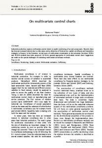
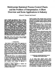
To calculate CLkernel , we may use a proper closed form which can be found in tables of integrals. However, from a practical point of view, it may not be efficient to use tables of integral every time when one wishes to calculate the control limits. In the present study we used the trapezoidal rule (Burden and Faires, 2000), one of the numerical integration methods that approximate the value of a definite integral and calculated CLkernel . The degree of approximation of the trapezoidal rule depends on the number of space points (trapezoids). If the number of space points is large, the true integration result may not be significantly different from the result derived from the trapezoidal rule. Figure 1 shows control limits from KDE-based T 2 control charts with different numbers of spaced points when the dataset follows the multivariate lognormal distribution. The result shows that the values of the control limits fluctuated but stabilized after 1,000 spaced points. The accuracy of the estimates derived also depends on choosing an appropriate smoothing parameter capable of compromising between oversmoothness and undersmoothness of the estimated kernel distribution (Silver, 1986). A number of methods are available to select an optimal smoothing parameter (Sheather and Jones, 1991). However, no consensus exists on the best method to satisfy all conditions. Figure 2 illustrates the control limits derived from a KDE-based T 2 control chart with different values of bandwidths in situations in which the dataset follows a multivariate lognormal distribution. The asterisk shown in Figure 2 6
represents the optimal bandwidth obtained using MATLAB Statistics Toolbox that uses an algorithm from pages 31-32 in Bowman and Azzalini (1997) .
2.3
Proposed Bootstrap Percentile Approach
As discussed above, KDE-based T 2 control charts require some effort to find the appropriate modeling parameters and to perform the numerical integration that calculates the area of the estimated kernel density. In particular, our experience was that if the distribution is highly skewed (which is often the case), calculations of the area of the tail region become less accurate. To avoid these cumbersome tasks, we propose in this study a bootstrap approach that can be considered an alternate way of KDE (but is easier to use in practical applications) to establish the control limits for T 2 control charts when the dataset is not multivariate normally distributed. The bootstrap technique is one of the most widely used resampling methods to determine statistical estimates when the population distribution is unknown (Efron and Tibshirani, 1993; Efron, 1979). The bootstrap approach is more convenient than KDE as a way to establish control limits because it does not involve any modeling process in specifying the parameters. Figure 3 illustrates an overview of the bootstrap procedure to calculate control limits, and it is summarized as follows: 1. Compute the T 2 statistics with n observations from an in-control dataset using (1). 2(i)
2(i)
2(i)
2. Let T1 , T2 , . . . , Tn
be a set of n T 2 values from ith bootstrap sample (i = 1, . . . , B)
randomly drawn from the initial T 2 statistics with replacement. In general, B is the large number (e.g., B > 1,000).
7
300
250
KDE CL
200
150
100
50
0
0
500
1000
1500
2000
Number of Spaced Points
Figure 1: Control limits from KDE-based T 2 control charts with different number of spaced points.
300 Optimal Bandwidth = 0.14521 250
KDE CL
200
150
100
50
0
0
0.1
0.2
0.3
0.4
0.5
Bandwidth
Figure 2: Control limits from KDE-based T 2 control charts with different bandwidths.
8
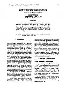
3. In each of B bootstrap samples, determine the 100·(1-α)th percentile value given a users-specified value α with a range between 0 and 1. 4. Determine the control limit by taking an average of B 100·(1-α)th percentile values (T¯2 100·(1−α) ). Note that statistics other than the average can be used (e.g., median). 5. Use the established control limit to monitor a new observation. That is, if the monitoring statistic of a new observation exceeds T¯2 100·(1−α) , we declare that specific observation as out of control. Although the bootstrap procedure does not involve an explicit process to determine parameters, the number of bootstrap samples used may affect the determination of control limits. Figure 4 illustrates various bootstrap control limits as determined by different numbers of bootstrap samples from 100 to 5,000. For each number of bootstrap samples, we calculated the control limit 1,000 times. The triangular in the figure indicates the average value of 1,000 control limits at each specified number of bootstrap samples. As expected, variability is greater when a small number of bootstrap samples are involved but stabilizes as the number of bootstrap samples increases. Determination of the appropriate number of bootstrap samples to use is not obvious. However, with reasonably large numbers of samples, the results vary little. The computational time required has been perceived as one of the disadvantages of the bootstrap technique, but this is not longer a significant issue because of the computing power currently available. Moreover, it is worth noting that the bootstrap tends to work better for statistics that are closer to being pivotal, such as the T 2 statistic that the we used in the present paper. However, the bootstrap might not work so well if the process mean is the statistic for the control chart.
9
3
Simulation Study
3.1
Simulation Setup
Simulation studies were conducted to evaluate the performance of the proposed bootstrapbased T 2 control chart and to compare it with the traditional T 2 and KDE-based T 2 control charts. One thousand bootstrap samples (B = 1, 000) were used in this experiment. For KDEbased T 2 control charts, we used the standard normal distribution as the kernel function. We generated 1,000 in-control observations (n = 1, 000) as a training set based on multivariate normal (N ), multivariate skew-normal (SN ), multivariate lognormal (LogN ), and multivariate gamma (Gam) distributions. Each dataset was characterized by three process · ¸ variables. We used µ = 0 0 0 to simulate the multivariate normal, multivariate skewnormal, and multivariate gamma distributions. In the multivariate lognormal distribution, µ · ¸ = 1 1 1 was used. Further, the following covariance matrix was used for the multivariate normal, multivariate skew-normal, and multivariate lognormal distributions: 1.00 0.70 0.60 Σ = 0.70 1.00 0.10 . 0.60 0.10 1.00 In the multivariate skew-normal distribution, different degrees of skewness (λ) were considered so as to observe the effects of these differences on the performance of the control charts. We used an R package (www.r-project.org) to generate multivariate skew-normal data. For illustrative purposes, Figure 5 shows two-dimensional skew-normal distributions with degrees of skewness from zero to three. The zero degree skew-normal distribution shows the regular normal distribution without any skewness. However, this figure also shows that as the degree of skewness increases, the simulated data become more skewed. For more details about the 10
Figure 3: An overview of the bootstrap procedure in calculating the control limits in T 2 control charts.
Mean of Bootstrap CL
52 50
Bootstrap CL
48 46 44 42 40 38 0
1000
2000
3000
4000
5000
Number of Bootstrap Samples
Figure 4: Control limits with different number of bootstrap samples.
11
multivariate skew-normal distribution, one can refer to Azzalini and Dalla Valle (1996). In the multivariate gamma distribution, the shape and scale of the parameters were specified as one.
3.2 3.2.1
Simulation Results Comparison of Control Limits
We generated two sets of 1,000 in-control observations. The first set of 1,000 in-control observations was used to determine the control limits of the T 2 control charts from the F distribution, KDE, and bootstrap percentile approaches. The second set of 1,000 in-control observations was monitored on the control charts, which were based on the control limits established by the first set of in-control observations. The control chart that produces a similar value for the actual false alarm rate and the assumed false alarm rate would be considered the better one. Figure 6 displays T 2 control charts from the second set of 1,000 in-control observations that use the normal distribution in conjunction with four different degrees of skewness. The control limits were computed using the F -distribution, KDE, and bootstrap percentile approaches. We specified a false alarm rate of 0.01. As illustrated, all three approaches yielded similar control limits in the multivariate normal distribution with zero skewness. As skewness (λ) increases, the control limits from the F -distribution tended to generate higher false alarm rates. However, the KDE and bootstrap percentiles controlled the assumed false alarm rates well. As can be seen from Figure 7, this behavior becomes much clearer in two nonnormal distributions (e.g., lognormal and gamma). In these, we specified a false alarm rate of 0.01 and generated three different control limits. The results clearly show that the F -distribution 12
approach failed to control the assumed false alarm rate and generated many false alarms. In contrast, the control limits determined by the KDE and bootstrap approaches produced similar values for the actual false alarm rate and for the assumed false alarm rate.
3.2.2
Comparison of In-Control Average Run Length
ARL is a performance measure that is widely used to evaluate control charts. In the present study, in-control ARL (ARL0 ) was used to compare the performance of the control charts. ARL0 is defined as the average number of observations required for the control chart to detect a change under the in-control process (Woodall and Montgomery, 1999). In this study, the average value of ARL0 was calculated from 10,000 replications. Under the normality assumption, the actual ARL0 of the T 2 control chart is expected to be the same as or close to the assumed ARL0 . Tables 1 ∼ 4 show the assumed ARL0 values and the actual ARL0 values as obtained by the F -distribution, KDE, and bootstrap percentile approaches in multivariatenormal situations in which different degrees of skewness were used. This figure shows that across the different approaches the actual ARL0 values are close to the assumed ARL0 values when skewness is zero. However, as the degree of skewness increases, the differences between the actual ARL0 , as determined by the F -distribution and the desired ARL0 , increases. In contrast, KDE and the bootstrap percentile approaches in skew-normal situations generated similar actual and assumed ARL0 results. As with skew-normal situations, in the multivariate lognormal case (Table 5)and the multivariate gamma case (6)the actual ARL0 values from the KDE and bootstrap percentile approaches are close to the assumed ARL0 values. Note that the average standard errors shown in parentheses in Tables 1 ∼ 6 are small enough to permit a meaningful conclusion.
13
4
4
3 3 2 2
X2
X
2
1 0
1
−1 0 −2 −1 −3 −4 −4
−3
−2
−1
0
1
2
3
−2 −2
4
X1
3
3
2
2
X2
2
X
4
1
0
−1
−1
1
2
3
2
3
4
5
1
0
0
1
(b) Skew-normal Distribution (λ = 1)
4
−1
0
X1
(a) Normal Distribution (λ = 0)
−2 −2
−1
4
X1
−2 −1.5
−1
−0.5
0
0.5
1
1.5
2
2.5
X1
(c) Skew-normal Distribution (λ = 2)
(d) Skew-normal Distribution (λ = 3)
Figure 5: The multivariate normal and multivariate skew-normal distributions with different degrees of skewness in two dimensions.
14
3
3.5
25
25 F−Dist CL KDE CL Bootstrap CL
F−Dist CL KDE CL Bootstrap CL
15
15
T
T
2
20
2
20
10
10
5
5
0
0
200
400
600
800
0
1000
0
200
Observation Number
400
600
800
1000
Observation Number
(a) Normal Distribution (λ = 0)
(b) Skew-normal Distribution (λ = 1)
25
25 F−Dist CL KDE CL Bootstrap CL
F−Dist CL KDE CL Bootstrap CL
15
15
T
T
2
20
2
20
10
10
5
5
0
0
200
400
600
800
1000
Observation Number
0
0
200
400
600
800
Observation Number
(c) Skew-normal Distribution (λ = 2)
(d) Skew-normal Distribution (λ = 3)
Figure 6: Control limits established by the F -distribution, KDE, and the proposed bootstrap percentile on the multivariate normal and multivariate skew-normal distributions under conditions of different degrees of skewness (α = 0.01).
15
1000
Table 1: ARL0 from the control limits established by using the F -distribution, KDE, and the bootstrap percentile approaches from 10,000 simulation runs based on the multivariate normal distribution (average standard errors are shown inside the parentheses). Case
α
Desired ARL0
F -dist
KDE
Bootstrap
N
0.01
100.000
101.980
103.950
99.962
(1.012)
(1.114)
(1.074)
51.542
51.850
50.143
(0.517)
(0.540)
(0.521)
33.736
33.965
32.726
(0.331)
(0.335)
(0.323)
25.053
25.560
24.677
(0.248)
(0.258)
(0.250)
20.301
20.443
19.808
(0.199)
(0.204)
(0.198)
16.906
17.120
16.628
(0.163)
(0.167)
(0.163)
14.323
14.469
14.046
(0.138)
(0.141)
(0.137)
12.629
12.764
12.418
(0.122)
(0.124)
(0.121)
11.026
11.162
10.818
(0.104)
(0.106)
(0.103)
10.111
10.207
9.924
(0.098)
(0.099)
(0.096)
0.02
0.03
0.04
0.05
0.06
0.07
0.08
0.09
0.10
50.000
33.333
25.000
20.000
16.667
14.286
12.500
11.111
10.000
16
Table 2: ARL0 from control limits established by using F -distribution, KDE, and bootstrap percentile approaches from 10,000 simulation runs based on the multivariate skew-normal distribution with λ = 1 (average standard errors are shown in parentheses). Case
α
Desired ARL0
F -dist
KDE
Bootstrap
SN (λ = 1)
0.01
100.000
81.724
103.200
100.12
(0.827)
(1.149)
(1.112)
45.059
50.804
49.413
(0.453)
(0.529)
(0.514)
31.369
34.184
33.056
(0.316)
(0.352)
(0.339)
23.606
24.933
24.364
(0.231)
(0.250)
(0.243)
19.610
20.636
20.012
(0.194)
(0.207)
(0.200)
16.101
16.558
16.118
(0.159)
(0.164)
(0.160)
14.210
14.568
14.182
(0.138)
(0.143)
(0.139)
12.534
12.72
12.377
(0.120)
(0.122)
(0.118)
11.253
11.415
11.075
(0.107)
(0.109)
(0.106)
9.932
10.07
9.7786
(0.096)
(0.098)
(0.095)
0.02
0.03
0.04
0.05
0.06
0.07
0.08
0.09
0.10
50.000
33.333
25.000
20.000
16.667
14.286
12.500
11.111
10.000
17
Table 3: ARL0 from control limits established by using the F -distribution, KDE, and bootstrap percentile approaches from 10,000 simulation runs based on the multivariate skewnormal distribution with λ = 2 (average standard errors are shown in parentheses). Case
α
Desired ARL0
F -dist
KDE
Bootstrap
SN (λ = 2)
0.01
100.000
71.901
101.45
98.821
(0.719)
(1.090)
(1.051)
41.846
51.772
50.562
(0.423)
(0.532)
(0.520)
29.587
33.850
32.944
(0.294)
(0.343)
(0.331)
23.089
25.483
24.897
(0.228)
(0.256)
(0.250)
19.019
20.370
19.894
(0.185)
(0.200)
(0.195)
16.137
16.944
16.512
(0.157)
(0.166)
(0.163)
13.977
14.467
14.146
(0.136)
(0.143)
(0.139)
12.338
12.642
12.277
(0.120)
(0.124)
(0.120)
11.007
11.141
10.859
(0.106)
(0.108)
(0.105)
10.018
10.074
9.806
(0.096)
(0.097)
(0.094)
0.02
0.03
0.04
0.05
0.06
0.07
0.08
0.09
0.10
50.000
33.333
25.000
20.000
16.667
14.286
12.500
11.111
10.000
18
Table 4: ARL0 from the control limits established by using F -distribution, KDE, and bootstrap percentile approaches from 10,000 simulation runs based on the multivariate skewnormal distribution with λ = 3 (average standard errors are shown in parentheses). Case
α
Desired ARL0
F -dist
KDE
Bootstrap
SN (λ = 3)
0.01
100.000
69.605
103.410
101.050
(0.692)
(1.106)
(1.076)
39.696
50.037
48.928
(0.402)
(0.591)
(0.509)
28.982
33.824
33.02
(0.287)
(0.347)
(0.338)
22.744
25.183
24.668
(0.229)
(0.256)
(0.251)
18.712
20.090
19.612
(0.185)
(0.197)
(0.193)
15.961
16.834
16.404
(0.156)
(0.164)
(0.160)
14.064
14.661
14.273
(0.137)
(0.143)
(0.139)
12.214
12.479
12.193
(0.119)
(0.121)
(0.118)
11.360
11.553
11.254
(0.110)
(0.112)
(0.108)
10.078
10.143
9.899
(0.096)
(0.097)
(0.094)
0.02
0.03
0.04
0.05
0.06
0.07
0.08
0.09
0.10
50.000
33.333
25.000
20.000
16.667
14.286
12.500
11.111
10.000
19
Table 5: ARL0 from control limits established by using F -distribution, KDE, and bootstrap percentile approaches from 10,000 simulation runs based on the multivariate lognormal distribution (average standard errors are shown in parentheses). Case
α
Desired ARL0
F -dist
KDE
Bootstrap
LogN
0.01
100.000
20.457
108.680
105.780
(0.208)
(1.251)
(1.142)
17.505
52.392
51.512
(0.172)
(0.562)
(0.527)
15.850
34.085
33.917
(0.155)
(0.349)
(0.342)
14.724
25.300
25.119
(0.143)
(0.272)
(0.251)
13.831
20.179
20.127
(0.137)
(0.201)
(0.200)
13.177
16.833
16.731
(0.130)
(0.167)
(0.163)
12.660
14.54
14.492
(0.126)
(0.145)
(0.145)
12.085
12.646
12.547
(0.117)
(0.123)
(0.121)
11.417
11.106
10.981
(0.111)
(0.108)
(0.106)
11.307
10.163
10.075
(0.110)
(0.099)
(0.098)
0.02
0.03
0.04
0.05
0.06
0.07
0.08
0.09
0.10
50.000
33.333
25.000
20.000
16.667
14.286
12.500
11.111
10.000
20
Table 6: ARL0 from control limits established by using F -distribution, KDE, and bootstrap percentile approaches from 10,000 simulation runs based on the multivariate gamma distribution (average standard errors are shown in parentheses). Case
α
Desired ARL0
F -dist
KDE
Bootstrap
Gam
0.01
100.000
20.939
105.650
103.050
(0.207)
(1.164)
(1.114)
16.995
50.437
50.169
(0.162)
(0.518)
(0.514)
14.572
33.472
33.338
(0.141)
(0.341)
(0.338)
13.253
25.142
25.147
(0.129)
(0.249)
(0.250)
12.215
20.214
20.105
(0.119)
(0.201)
(0.200)
11.158
16.675
16.563
(0.107)
(0.163)
(0.162)
10.452
14.210
14.132
(0.100)
(0.139)
(0.138)
10.054
12.604
12.537
(0.097)
(0.122)
(0.121)
9.298
11.041
10.982
(0.089)
(0.109)
(0.108)
8.91
9.965
9.909
(0.086)
(0.097)
(0.096)
0.02
0.03
0.04
0.05
0.06
0.07
0.08
0.09
0.10
50.000
33.333
25.000
20.000
16.667
14.286
12.500
11.111
10.000
21
4
Case Study
The proposed bootstrap-based T 2 control chart was implemented by applying it as a case study to a real multivariate process in a power generation company. The ultimate goal of this case study was to develop an efficient monitoring and diagnostic tool for early detection of abnormal behavior and performance degradation in a power company. The dataset contains 2,000 observations collected over a period in which each observation was characterized by 18 process variables. Further, the power company’s process experts confirmed that this dataset is in control and stable. To check its multivariate normality, we conducted Royston’s H test (Royston, 1983). The p-value, which measures the plausibility that the dataset follows multivariate normal distribution, was almost zero. This strongly indicates that this dataset does not come from the multivariate normal distribution. Figure 8 shows the T 2 control charts whose control limits were estimated by the F distribution, KDE, and proposed bootstrap approaches with a false alarm rate (α) of 0.01. As shown, the actual false alarm rates from both the KDE and bootstrap percentile approaches are 0.0095, which is similar to the assumed false alarm rate (0.01). On the other hand, the actual false alarm rate from the F -distribution is 0.052, resulting in a lower control limit and a higher false alarm rate. This demonstrates the effectiveness of the proposed bootstrap-based T 2 control chart in a real situation in which the process does not follow the multivariate normal distribution.
22
180
55 F−Dist CL KDE CL Bootstrap CL
160
F−Dist CL KDE CL Bootstrap CL
50 45
140 40 120
35 2
30
T
T
2
100
25
80
20
60
15 40 10 20 0
5 0
200
400
600
800
1000
0
0
200
400
Observation Number
600
800
Observation Number
(a) Lognormal Distribution Case
(b) Gamma Distribution Case
Figure 7: Control limits established by the F -distribution, KDE, and the proposed bootstrap percentile on the multivariate lognormal and the multivariate gamma distributions (α = 0.01).
F−Dist CL KDE CL Bootstrap CL
120
100
T
2
80
60
40
20
0
0
500
1000
1500
2000
Observation Number
Figure 8: Control limits established by the F -distribution, KDE, and proposed bootstrap percentile approach on the real dataset.
23
1000
5
Concluding Remarks
This study proposed a bootstrap approach as a way to determine the control limits of a T 2 control chart when the observations do not follow a normal distribution. KDE is an existing method used to establish the control limits of T 2 control charts in nonnormal situations. We want to emphasize again that the purpose of the present study is not to outperform the KDE approach. Rather, we proposed an alternate way for a KDE-based T 2 control chart to deal with nonnormal situations. Nevertheless, the proposed bootstrap-based T 2 chart is a model-free approach and thus easier to implement without recourse to a strong statistical background. The simulation study showed that the proposed bootstrap-based T 2 control charts outperformed the traditional T 2 control charts in both skew-normal and nonnormal cases and were comparable in ARL performance with the KDE-based T 2 control charts. With normally distributed data, all three approaches produced comparable ARL performance. This result clearly indicates that the proposed bootstrap-based control chart is efficient in both normal and nonnormal situations. Further, we used the proposed control chart to monitor a real multivariate process in a power generation company and obtained results consistent with the simulation study. We believe that the fundamental value of the present study includes the integration of the bootstrap method with traditional Hotelling’s T 2 control charts to extend their applicability in nonnormal situations.
References Azzalini A. and Dalla Valle A. (1996) The multivariate skew-normal distribution. Biometrika, 83, pp.715–726.
24
Bajgier, S.M. (1992) The Use of Bootstrapping to Construct Limits on Control Charts. Proceedings of the Decision Science Institute, San Diego, CA, 1611–1613 Bersimis, S., Psarakis, S. and Panaretos, J. (2006) Multivariate statistical process control charts: an overview. Quality & Reliability Engineering International, 23(5), 517–543. Bowman, A.W., and Azzalini, A. (1997) Applied Smoothing Techniques for Data Analysis. Oxford University Press, 31–32. Burden, R.L., and Faires, J.D. (2000) Numerical Analysis. Books Cole, New York. Chakraborti, S., Van Der Laan, P. and Bakir, S.T. (2001) Nonparametric control chart: an overview and some results. Journal of Quality Technology, 33(3), 304–315. Chou, Y-M., Mason, R.L., and Young J.C. (2001) The Control Chart for Individual Observations from A Multivariate Non-normal Distribution. Communications in Statistics– Simulation and Computation, 30(8–9), 1937–1949. Efron, B. (1979) Bootstrap Methods: Another Look at the Jacknife. The Annals of Statistics, 7(1), 1–26. Efron, B. and Tibshirani, R. (1993) An Introduction to the Bootstrap. Chapman & Hall/CRC, Boca Raton, FL. Hotelling, H. (1947) Multivariate Quality Control. in Techniques of Statistical Analysis, Eisenhart, C., Hastay, M.W., and Wills, W.A. (eds), McGraw-Hill, New York, NY, pp. 111–184. Jones, L.A. and Woodall, W.H. (1998) The Performance of Bootstrap Control Charts. Journal of Quality Technology, 30, 362–375.
25
Lowry, C.A. and Montgomery, D.C. (1995) A review of multivariate control charts. IIE Transactions, 27(6), 800–810. Lio, Y.L. and Park, C. (2008) A Bootstrap Control Chart for Birnbaum-Saunders Percentiles. Quality and Reliability Engineering International, 24, 585–600. Liu, R.Y. and Tang, J. (1996) Control Charts for Dependent and Independent Measurements Based on the Bootstrap. Journal of the American Statistical Association, 91, 1694–1700. Mason, R.L. and Young, J.C. (2002) Multivariate Statistical Process Control with Industrial Applications. American Statistical Association and Society for Industrial and Applied Mathematics, Philadelphia, PA. Montgomery, D.C. (2005) Introduction to Statistical Quality Control, fifth edition. Wiley, New York, NY. Park, H.I. (2009) Median Control Charts Based on Bootstrap Method. Communications in Statistics–Simulation and Computation, 38, 558–570 Polansky, A.M.(2005) A general framework for constructing control charts. Quality and Reliability Engineering International, 21, 633–653. Royston, J.P. (1983) Some techniques for assessing multivariate normality based on the Shapiro-Wilk W. Applied Statistics, 32(2), 121–133. Seppala, T., Moskowitz, H., Plante, R., and Tang J. (1995) Statistical Process Control via the Subgroup Bootstrap. Journal of Quality Technology, 27, 139–153. Sheather, S.J. and Jones, M.C. (1991) A Reliable Databased Bandwidth Selection Method for
26
Method Kernel Density Estimation. Journal of Royal Statistical Society Series B, 53(3), 683–690. Silverman, B.W. (1986) Density Esimation for Statistics and Data Analysis. Chapman and Hall, London, United Kingdom. Tracy, N.D., Young, J.C., and Mason, R.L. (1992) Multivariate Control Charts for Individual Observations. Journal of Quality Technology, 25, 161–169. Woodall, W.H. (2000) Controversies and contradictions in statistical process control. Journal of Quality Technology, 32(4), 341–350. Woodall, W.H. and Montgomery, D.C. (1999) Research issues and ideas in statistical process control. Journal of Quality Technology, 31(4), 376–386.
27