Performance of control charts for autoregressive conditional ...

Journal of A pplied Statistics, Vol. 26, N o. 6, 1999, 701± 714

Perform ance of control charts for autoregressive conditional heteroscedastic processes

1

2

1

YU E FA NG & JOHN ZH ANG , Lundquist C ollege of B usiness, University of 2 Oregon, USA and Department of M athematics, Indiana University of Pennsylvania, USA

This paper examines the robustness of control schemes to data conditional heteroscedasticity. Overall, the results show that the control schemes which do not account for heteroscedasticity fail in providing reliable information on the status of the process. Consequently, incorrect conclusions will be drawn by applying these procedures in the presence of data conditional heteroscedasticity. C ontrol charts with time-var ying control limits are shown to be useful in that context. AB STRACT

1 Introduction Traditional control charts, such as the Shew hart, cumulative sum (C USUM ) and exp onentially weighted m oving average (EW M A) control schem es, have been widely used in statistical process control (SPC). They serve as on-line SPC procedures to m onitor process stability, to detect assignable variation, or to forecast process m ovem ents in industrial processes and other applications. A typical control chart is constructed from a sam ple collected when the process is in control. To determ ine the param eters of control charts, assumptions about the data generated by the process have to be m ade. In standard SPC applications, a state of control is identi® ed with a process generating independent and identically distributed (iid) norm al random variables. In practice, it is often diý cult to attain a state of control in this strict sense. In situations where the norm ality assum ption is violated or the independence assum ption is not satis® ed, the control charts based on the iid assum ptions m ay be Correspondence: Y. Fang, Lundquist College of Business, U niversity of Oregon, Eugene, OR 97403 , U SA. Tel: 541 346 3265 ; E-m ail: yfang@ darkwing.uoregon.edu 0266-476 3/99/060701-1 4

1999 Taylor & Francis Ltd

702

Y. Fang & J. Zhang

ineþ ective and inappropriate. It is well known that distributions with heavier tails m ay increase the presence of outliers in the data. However, in general, the control charts are not sensitive to the norm ality assum ption and work reasonably well unless the population is markedly non-norm al. If data are not independent, then the control charts which do not take account of autocorrelation could wrongly infer that the process is in control or signal that an assignable cause m ight have occurred. M ore sophisticated control schem es have been proposed for serially correlated observations based on the autoregressive m oving average (ARMA) m odels (see, for exam ple, Alwan & Roberts, 1988; Harris & Ross, 1991; Wardell et al., 1994). AR M A (Box & Jenkins, 1994) processes are linear m odels. If the disturbance term is assum ed to be norm ally distributed, then the analysis of ARM A processes is within the Gaussian fram ework. We can regard the process based on ARMA m odels as `in control’ in a broader senseÐ a sense that goes beyond the sim ple benchm ark of iid random variables. In order to obtain a better understanding of the process, it is often required to m odify the standard SPC procedures so that the m odel assum ptions are approxim ately satis® ed and a rigorous analysis is possible. For exam ple, serial correlation, seasonality, m issing values and non-constant variance are som e com m on features in environm ental, biological and chem ical data (Berthouex et al., 1978). In order to apply SPC charts to those data, a wider class of stochastic m odels m ay be required. In this paper, we extend the study of SPC procedures to som e non-linear processes. M ore speci® cally, we investigate the robustness of control charts to data conditional heteroscedasticity. In som e applications, data conditional heteroscedasticity is com m on and is often associated with processes that have heavy tails and variability clusters. For example, C uthbertson and Gasparro (1993) studied m anufacturing inventories and found that the general autoregressive conditional heteroscedastic (G AR C H) m odel is consistent w ith existing theories and with U K data. Weiss (1984) analyzed 16 U S econom ic series from the C itibank Econom ic D atabase and ® tted AR CH -type m odels to the data w ith varying degrees of success. Heteroscedasticity has an important consequence for control problem s. In this paper, we provide evidence that the control schem es, w hich do not account for heteroscedasticity, are not robust to data conditional heteroscedasticity. O ur study indicates that, in general, the conventional calculated control lim its are invalid. T he in-control average run length (AR L) falls substantially and the m agnitude depends on the param eters of conditional variance processes. We also develop a sim ple control scheme with tim e-varying control lim its and show that the proposed procedure is useful in dealing with conditional heteroscedasticity data. To facilitate the study, we assum e that the processes can be described by either G AR C H or ARM A± ARCH processes. G AR C H m odels represent one type of nonlinear model, while the conditional variance varies over tim e; ARM A± ARCH processes are ARM A m odels with ARCH errors (see D e G ooijer and Kum ar (1992) for a review of non-linear m odels, and Tong (1990) for further discussion on the subject). The non-linearity stem s from the conditional heteroscedasticity of the disturbance term . G AR C H and AR M A± AR CH processes have been successfully applied in m any tim e series (see Bollerslev et al. (1992) for a survey). T here are various reasons for the presence of conditional heteroscedasticity in the observed sequence. O ne reason is that any changes in the tim escale of data sampling may create AR C H eþ ects in the observed tim e series (Stock, 1988). Am ong a w ide variety of control schem es, the Shewhart, C USUM and EW MA

Control charts and conditional heteroscedasticity

703

schem es are basic and popular. All three charts have been constructed under the norm ality and independence assum ptions. They share som e com m on appealing aspects, such as being easy to set up, im plem ent and interpret. We will focus on the EW MA chart. The conclusions for the Shew hart and CU SU M charts are sim ilar and the results are not reported in this paper. This paper is organized as follow s. Section 2 describes the GARCH (1,1) m odel, which ser ves as a data generator. In Section 3, the perform ance of the EW M A control schem e is evaluated in the presence of data conditional heteroscedasticity. T he AR Ls, as a m easurem ent of perform ance, are assessed through a sim ulation study, given that a single step shift in the process mean occurs. An adjusted control schem e with tim e-varying control lim its subject to data conditional heteroscedasticity is discussed in Section 4. Section 5 extends our discussion to the control schem es designed for serially correlated data. C oncluding rem arks are presented in Section 6.

2 G A RCH (1,1) m odel A w ide variety of m odels based on the ARCH type were developed by Engle (1982) and were generalized by Bollerslev (1986). In this section, we consider the G AR C H(1,1) model. T he G ARCH(1,1) m odel considers a stochastic process y t in equidistant discrete time t. T he distribution of observations { y t } is speci® ed by the distribution of y t conditional on its past values y t2 1 . W ithout loss of generality, the process m ean, when the process is in control, is assum ed to be zero. T he model can be form ulated as yt 5

r te

(1)

t

and 2 t 5

r

c

+ a y 2t 2

1

+

2 t2 1

b r

(2)

where the param eters c , a , b > 0, and a + b < 1. { e t } are iid standard norm al. T he param eters a and b are particularly interesting, because they provide inform ation about the persistence of temporal shocks. The conditional distribution of y t is normal with m ean zero and standard deviation r t . However, the unconditional distribution of y t is not of any standard form . By the usual ARM A analog, the process is weakly stationary with m ean zero and constant unconditional variance r

2

º

Var( y t ) 5

c

12

a 2 b

(3)

T he existence of higher m om ents of y t depends on the levels of both a and b . T he distribution of y t is sym m etric, since all the odd mom ents of y t are zero. T he kurtosis of y t , i.e. j , is given by j º

E [ y t 2 E ( y t )] 5 Var 2 ( y t ) 4

3 2 3 (a + b )2 1 2 3a 2 2 b 2 2 2a b

(4)

T he kurtosis exists only for (1 2 3 a 2 2 b 2 2 2 a b ) > 0 w ith a , b > 0. In equation (4), j in (4) is greater than 3 if either a or b is greater than zero; therefore, the m odel yields observations with heavier tails than those of a norm al distribution.

704

Y. Fang & J. Zhang

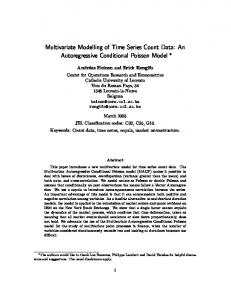
F IG. 1. The regions in which the variance r

2

and the kurtosis j are well de® ned.

2

One can verify equation (4) by applying the fact that y t is ARM A(1,1), i.e. 2

yt 5 c

+ ( a + b ) y 2t2 1 + a t 2

b a t2

1

where a t 5 r (e 2 1) is white noise (Har vey, 1993). In the interests of brevity, we do not include the detailed com putation here. Figure 1 shows the regions of a and b in which the variance and the kurtosis of y t exist. 2 t

2 t

3 E W M A schem e in the presence of data conditional heteroscedasticity T he general m odel of control charts consists of the center line l , which is the equilibrium level of som e quality characteristic of interest; the upper control lim its (U CL) and the lower control lim its (LC L), which have the same distance from the center line, exp ressed in standard deviation units of the observed sequence r y . We have Control limits 5

l 6

kLr

zt

(5)

where k is a predeterm ined constant and the value of the param eter L depends on the design of the chart. In the EW M A case, z t 5 k y t + (1 2 k )z t2 1 and L5

{

22

}

1/2

k k

[1 2

(1 2

2t

k ) ]

where k is the sm oothing param eter, w hich is the weight assigned to the last observation. We will have that l 5 0 in equation (5), since the process mean is assumed to be zero w hen the process is in control. Theoretical derivations of the AR Ls for G AR C H processes are diý cult. We perform simulation experim ents for AR Ls when the process m ean has shifted by q r y for som e non-negative param eter q . If q 5 0, then the process is in control. D ata are generated by the GARCH(1,1) m odel de® ned in equations (1) and (2). T he perform ance of the EW M A scheme is evaluated on the param eter space spanned by a and b . The levels of a and b are in the interval [0.0, 1.0) with increment 0.1. Im posing the weakly stationary condition a + b < 1 im plies that


705

AR Ls are calculated only on half the a and b space. We assum e that r 2y 5 1 for all sim ulations; therefore, the param eter c 5 1 2 a 2 b from equation (3). To assess the robustness of the EW MA scheme to the data conditional heteroscedasticity, we perform sim ulation experim ents for the sm oothing param eter k 5 0.1 and 0.3. The m ultiplier k in equation (5) is chosen so that AR L 5 370 in the case of no shift in the process m ean and no data conditional heteroscedasticity. For exam ple, when k 5 0.1, k 5 2.715. If k 5 0.3, then k increases to be approxim ately 2.928. M ore values of k for diþ erent in-control AR L s can be found in Lucas and Saccucci (1990). T he process is initialized at the in-control value and the process m ean shifts im m ediately after the ® rst observation. All sim ulations are based on 10 000 replications. Figures 2 ± 5 report the sim ulation results for k 5 0.1 when q 5 0.0, 0.5, 1.0 and

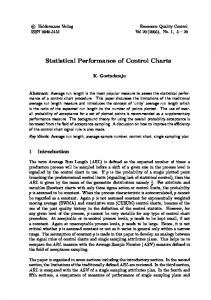
F IG. 2. Contour plot of the AR L for the in-control EWM A with k 5

F IG. 3. Contour plot for the EWM A with k 5

0.1.

0.1 , when the process has shifted by half a standard deviation.

706

Y. Fang & J. Zhang

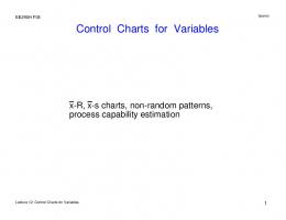
F IG. 4. Contour plot of the AR L with k 5

0.1, w hen the process has shifted by one standard deviation.

F IG. 5. Contour plot of the AR L with k 5

0.1, when the process has shifted by three standard deviations.

3.0 respectively. T he AR L for an in-control EW M A ( q 5 0.0) is shown in Fig. 2. T he AR L is less than 370 for m ost of the a and b com binations, except for the regions w ith a » 0 or a + b » 1. A signi® cant reducation in AR L occurs if a is not close to zero or a + b is not close to unity. The lowest AR L is about 230, w hich is equivalent to a reduction of 37.84%. In general, the values of the AR L depend on both a and b . H owever, a has m ore im pact on AR Ls than does b . The kurtosis of y t , i.e. j , plays an important role and the cur ve 2 2 1 2 3 a 2 b 2 2 a b 5 0 divides the a and b space into two non-overlapping areas. If 2 2 1 2 3 a 2 b 2 2 a b > 0, then j exists. AR L 5 370 when the observations are iid norm al ( a 5 b 5 0). As a and b increase, j > 3. Consequently, the AR L decreases, as a result of the conditional heteroscedasticity eþ ects. The behavior of the AR L is interesting w hen 1 2 3 a 2 2 b 2 2 2 a b < 0. In this case, the kurtosis of y t does not exist. However, the AR L does not continue to drop as


707

increase; instead, rather surprisingly, it increases as a + b approaches unity. T he lowest AR Ls settle around the curve of 1 2 3 a 2 2 b 2 2 2 a b 5 0. For exam ple, if b 5 0, then the kurtosis of y t is given by a and b

{ 5

j 5

3(1 2 a

2

) /(1 2

3,

3 a ) > 3, 2

does not exist,

a 5

0

a < (1/3)

1/2

a >

1/2

(1/3)

T he AR L ® rst decreases and then increases when a varies from zero to unity. The lowest AR L is at about 222.7 w hen a is around (1/3) 1/2 5 0.577. In order to understand the behavior of the AR L when 1 2 3 a 2 2 b 2 2 2 a b < 0, let us consider an extrem e case where a + b » 1. W hen we set a + b 5 1, the G AR C H (1,1) model in equations (1) and (2) becom es an integrated G ARCH (IG ARCH) m odel. T he IG AR C H process is no longer weakly stationary, since it does not have a ® nite second m ovement. However, the IG ARC H process is strictly stationary and has the strange property that, no m atter w hat the starting point, r 2t collapses to zero almost de® nitely (Nelson, 1990). H ence, the observed series eþ ectively disappears. As a + b approaches unity, the observed series behaves m ore like an IGARCH process. T he conditional heteroscedasticity eþ ects decrease and the AR L clim bs back to and even beyond the nominal level (370) for som e values of a and b . Figures 3 ± 5 show the eþ ects on the AR Ls when the process m ean has shifted. Again, the AR Ls are m ore likely in¯ uenced by a than by b . Surprisingly, we ® nd that the AR Ls have a strong tendency to increase as a increases, especially in the cases in which q 5 1.0 and q 5 3.0. The m agnitude of the increment of the AR Ls depends on the level of the shift param eter q . Figures 6 ± 9 report the sim ulation results for k 5 0.3 when q 5 0.0, 0.5, 1.0 and 3.0 respectively. T he AR L for an in-control EW MA ( q 5 0.0) is shown in Fig. 6 and indicates a very sim ilar pattern as for the case k 5 0.1 when a and b vary. T he AR Ls are less than 370 for the m ajority of a and b . T he reduction in the AR Ls is signi® cant when a is between 0.2 and 0.8 Figures 7 ± 9 show the eþ ects on the AR Ls when the process m ean has shifted.

F IG. 6. Contour plot of the AR L for the in-control EWM A with k 5

0.3.

708

Y. Fang & J. Zhang

F IG. 7. Contour plot of the AR L for the EWM A with k 5 0.3, when the process has shifted by half a standard deviation.

F IG. 8. Contour plot of the AR L for the EW MA with k 5 0.3, when the process has shifted by one standard deviation.

U nlike the results for k 5 0.1, the AR Ls for q 5 0.5 and q 5 1.0 are not monotonic increasing functions of a . Instead, they depend on the levels of both a and b . T he m onotonic increasing phenom enon of the AR L that we observed when k 5 0.1 arises only for q 5 3.0. In summ ary, the EW MAs w hich do not account for heteroscedasticity are generally not robust to data conditional heteroscedasticity. The fourth m oment of y t , i.e. j , plays an im portant role in the determ ination of the AR Ls. Overall, the level of a has m ore impact on the AR Ls than does the level of b . W hen the process is in control, the EW MAs w ith both k 5 0.1 and k 5 0.3 oþ er higher out-of-control false alarm rates than those for the data without conditional heteroscedasticity. W hen the process is in control, the AR Ls are in the range 150 ± 370 for m ost of a


709

F IG. 9. Contour plot of the AR L for the EW MA with k 5 0.3 , when the process has shifted by three standard deviations.

and b . The reduction in the AR L is m ore signi® cant for k 5 0.3 than is that for k 5 0.1. H owever, when the process is out of control, the EW M As w ith k 5 0.1 are less sensitive to m ean shifts of all three levels com pared with the results for the data w ithout conditional heteroscedasticity. In contrast to the case of k 5 0.1, when the process is out of control, in general, the control schem e with k 5 0.3 is m ore sensitive to a small or a m edian m ean shift and is less sensitive to a large m ean shift com pared w ith the result for data without conditional heteroscedasticity.

4 C ontrol charts with tim e-var ying control lim its Although the GARCH m odel de® ned in equations (1) and (2) im plies that the unconditional variance of { y t } is a constant, the conditional variance of { y t } could change over time. The m odel for the tem poral dependence in conditional second m om ents suggests that tim e-varying control lim its should be appropriate. The setup in equation (2) allow s for using past information to construct the conditional variance of the process as an alternative to constant control lim it schemes. We suggest that the control lim its for the EW M A schem e have the form at l 6

Control lim its 5 where r

2 zt

is the conditional variance of z t 5 r 2

2 zt 5

k

2

t2

1

R

0

j5

(1 2

2j

k ) r

k yt 2 t2 j

kr

+ (1 2

+ (1 2

(7)

zt

k )z t2 2t

k ) r

1

and is given by

2 0

(8) 2

T he sequence { r t } depends on { y t } and the initial value r 0 . Its dynam ic is 2 determ ined by equation (2). We take r 0 to be unity, so that the unconditional variance of y is unity, as we did in the previous section. To illustrate control schem es with time-var ying control lim its, we use a sequence of sim ulated observations generated by equations (1) and (2) with param eters a 5 0.4 and b 5 0.0. Som e 100 z t term s are calculated and plotted with two diþ erent

710

Y. Fang & J. Zhang

1.0 0.5 0.0 ± 0.5 ± 1.0

0

50

100

150

200

150

200

(a) 1.0 0.5 0.0 ± 0.5 ± 1.0

0

50

100 (b)

F IG. 10. Sim ulated {z t } t 2 1 from y t 5 r t e t and r t 5 0.6 + 0.4 yt 2 1( k 5 0.1): (a) with constant control lim its (equation (5)); (b) with tim e-varying control lim its based on equations (7) and (8). 100

2

2

control schem es (see F ig. 10). O ne schem e has constant control lim its according to equation (5) and the other schem e uses tim e-varying control lim its based on equations (7) and (8). T he control schem e with tim e-varying control lim its utilizes the available inform ation and constantly upg rades the estim ation on the process variability. T he control schem e with tim e-varying control lim its is insensitive to data conditional heteroscedasticity, so creates fewer false out-of-control alarm s. To evaluate the perform ance of the proposed control schemes with tim e-var ying control lim its, we compute AR Ls according to the control lim its determ ined by equations (7) and (8), as well as AR Ls based on a `two-in-a-row ’ rule for com parison. T he two-in-a-row control procedure is used to detect problem s in control with heavier-tailed observations than norm al. Two successive observations in a row which are outside the lim its are considered to represent an out-of-control signal. T he two-in-a-row procedure is insensitive to excess variability caused by occasional outliers (Lucas & Saccucci, 1990). Since b has less in¯ uence on AR Ls than does a , b is taken to be zero in order to sim plify the evaluation. The param eter a is set equal to 0.1, 0.2, . . . , 0.9. We only report the results for the EW M A w ith k 5 0.1. Sim ilar conclusions can be m ade for EW M As w ith other k values. Again, the control lim its are based on a zero-state in-control AR L 5 370, as in Section 3. Figures 11 ± 13 report the AR Ls for EW M As w ith tim e-varying control lim its and schem es based on the two-in-a-row control rule. For a m oderate or large shift of the process m ean ( q 5 1.0 or 3.0), the schem e w ith time-varying control lim its outperforms the charts based on the two-in-a-row rule. For a sm all deviation of the process m ean ( q 5 0.5), the performances of the two control schem es are about the sam e, except that the scheme with tim e-var ying control lim its perform s poorly as a approaches unity.

Control charts and conditional heteroscedasticity 40

711

Time-varying limits Two-in-a-row

35

30

25

0.1

0.2 0.3

0.4

0.5

0.6

0.7

0.8

0.9

a F IG. 11. The AR Ls for EW MAs when the process m ean has shifted half standard deviation. b 5 j values are based on zero-state in-control APL 5 370.

13

0 and

Time-varying limits Two-in-a-row

12

11

10

9

0.1

0.2 0.3

0.4

0.5

0.6

0.7

0.8

0.9

a F IG. 12. T he AR Ls for EWM As when the process mean has shifted one standard deviation. b 5 j values are based on zero-state in-control AR L 5 370.

0 and

Overall, the control schem e w ith tim e-varying control lim its is found to perform better than does the schem e based on the two-in-a-row rule, except for the case where a is close to unity and q is relatively sm all. Other control schemes based on high m om ents, such as kurtosis, m ay be instructive and useful in som e applications. H owever, m ore sophisticated procedures m ay be diý cult to interpret and im plem ent.

712

Y. Fang & J. Zhang 5 Time-varying limits Two-in-a-row

4

3

2

0.1

0.2 0.3

0.4

0.5

0.6

0.7

0.8

0.9

a F IG. 13. The AR Ls for EW M As when the process m ean has shifted three standard deviations. b 5 and j values are based on zero-state in-control AR L 5 370.

0

5 C ontrol schem es designed for serially correlated obser vations In this section, we extend the discussion to the case of serially correlated obser vation sequences. The presence of serial correlation in the observation sequence m ay cause excessive variability and, consequently, the traditional control charts, such as the Shewhart, C USUM or EW M A schemes, becom e m eaningless. One approach to m onitor the serial correlated data is to ® t the data to a structure m odel and exam ine the residuals or the one-step-ahead forecast error, instead of the original data sequence. To m odel both serial correlation and data heteroscedasticity, the com bined ARM A± ARCH models are useful. AR M A± AR C H m odels are a natural extension of ARM A m odels which allow y t to have tim e-varying conditional second mom ents. For example, ARM A(1,1)± ARCH (1) can be w ritten as yt 2

(1 2

u yt 5

u )l + e t 2

h e

t2

(9)

1

where 2 t 5

r

E (e t ½ e 2

t2

1

,e

t2

2

, . .. )5

+ a y 2t2 c

1

(10)

T he process de® ned by equations (9) and (10) has m ean l and variance Var( y t ) 5

(1 + h 12

u

2

2

2

2

a (1

2 u h )c

+ h

2

2

2u h )

(11)

As the case without data conditional heteroscedasticity, one approach to data with both serial correlation and ARCH error structure is to ® t the observation sequence to AR M A m odels and then analyze the residuals by applying control schem es with tim e-varying control lim its as discussed in Section 4.


713

6 C onclusions O ur study indicates that control schemes which do not account for heteroscedasticity are not robust to data heteroscedasticity. In general, the in-control AR Ls fall substantially if data conditional heteroscedasticity is present, and the m agnitude depends on the kurtosis of the obser ved process. The control scheme with tim evar ying control lim its is introduced and the perform ance is evaluated against the alternative schem e based on the two-in-a-row rule. The M onte C arlo evidence suggests that the control schem e with tim e-var ying control limits works well, m aking it a useful tool in the presence of heteroscedasticity. AR C H-type m odels are non-linear m odels which include as special cases linear processes such as white noise and ARM A process. M axim um -likelihood estim ation procedures can be applied to the GARCH and ARM A± ARCH m odels, and the algorithm developed by Berndt et al. (1974) provides a convenient method of com putation. M ore details m ay be found, for exam ple, in E ngle (1982), Weiss (1984, 1986) and Bollerslev (1986). Although we have selected ARC H-type m odels to illustrate SPC procedures in the non-linear settings, in practice, the speci® c application will dictate w hich linear and /or non-linear m odel m ight be appropriate. T he idea proposed in this paper can be extended to deal with other form s of nonlinearity. It becom es clear that the m odel chosen to ® t the data is im portant and any m odel m isspeci® cation will result in false signals of the state of the process. T hat topic is beyond the scope of the discussion of this paper and readers interested in a com prehensive treatm ent of it are referred to the literature, such as Weiss (1986), Bollerslev et al. (1993) and Tiao and T say (1994).

Acknowledgem ents T he authors thank Frederick W. M organ, Gopal K. K anji (the editor) and the referee for helpful com m ents and suggestions.

R EFER EN C ES A LWAN, L. C. & R OBERTS, H. V. (1988 ) T ime series m odeling for statistical process control, Journal of B usiness & Economic Statistics, 6, pp. 87 ± 95. B ERNDT, E. R., H ALL, B. H ., H ALL, B. E. & H AUSMAN, J. A. (1974 ) Estim ation and inference in nonlinear structural m odels, Annals of Economic and Social Measurement, 4, pp. 653 ± 665. B ERTHOUEX, P. M ., H UNTER, W. G. & P ALLESEN, L. (1978 ) Monitoring sewage treatm ent plants: Som e quality control aspects, Journal of Quality Technology, 10, pp. 139 ± 149. B OLLERSLEV, T. (1986 ) Generalized autoregressive conditional heteroscedasticity, Journal of Econometrics, 31, pp. 307 ± 327 . B OLLERSLEV, T., C HOU, Y. & K RONER, K. F. (1992 ) ARCH models in ® nance: A review of theory and evidence, Jour nal of Econometrics, 52, pp. 5 ± 59. B OLLERSLEV, T., E NGLE, R. F. & N ELSON, D. B. (1993 ) ARCH models. In: R. F. E NGLE & D. M CF ADDEN (E ds), Handbook of Econometrics, Vol. 4, Chapter 49, pp. 2959 ± 3038 (Amsterdam , NorthH olland). B OX, G. E. P., J ENKINS, G. M . & R EINSEL, G. C. (1994) Time Series Analysis: Forecasting and Control (Englewood Cliþ s, NJ, Prentice Hall). C UTHBERTSON, K. & G ASPARRO, D. (1993 ) The determ inants of manufacturing inventories in the U K, The Economic Jour nal, 103, pp. 1479 ± 1492. D E G OOIJER, J. G. & K UMAR, K. (1992 ) Some recent developments in non-linear tim e series m odeling, testing, and forecasting, International Journal of Forecasting, 8, pp. 135 ± 156 . E NGLE, R. F. (1982 ) Autoregressive conditional heteroscedasticity with estim ates of the variance of U K in¯ ation, Econometrica, 50, pp. 987 ± 1007.

714

Y. Fang & J. Zhang

H ARRIS, T. J. & R OSS, W. H. (1991 ) Statistical process control procedures for correlated observations, The Canadian Journal of Chemical Engineering, 69, pp. 48 ± 57. H ARVEY, A. C. (1993) Time Series M odels (C ambridge, M A, MIT Press). L UCAS, J. M . & S ACCUCCI , M. S. (1990 ) Exponentially weighted m oving average control schem es: Properties and enhancements, Technometrics, 32, pp. 1 ± 12. N ELSON, D. B. (1990 ) Stationarity and persistence in the G ARCH (1,1) m odel, Technometrics, 32, pp. 1 ± 12. S TOCK, J. H. (1988 ) Estimating continuous-tim e processes subject to tim e deform ation, Journal of the Am erican Statistical Association, 83, pp. 77 ± 85. T IAO, G. C. & TSAY, R. S. (1994 ) Som e advances in non-linear and adaptive m odeling in time-series, Journal of Forecasting, 13, pp. 109 ± 131. T ONG, H. (1990) Non-linear Time Ser ies: A Dynamic System Approach (O xford, Clarendon Press). W ARDELL, D. G., M OSKOWITZ, H . & P LANTE, R. D. (1994 ) Run-length distributions of special-cause control charts for correlated processes, Technometrics, 36, pp. 3 ± 27. W EISS, A. A. (1984 ) ARM A models with ARCH errors, Journal of Time Series A nalysis, 5, pp. 129 ± 143. W EISS, A. A. (1986 ) ARCH and bilinear tim e series m odels: Comparison and combination, Journal of B usiness & Economic Statistics, 4, pp. 59 ± 70.