Bootstrapping Graph Convolutional Neural Networks for Autism Spectrum Disorder Classification Rushil Anirudh
[email protected]
arXiv:1704.07487v1 [stat.ML] 24 Apr 2017
Center for Applied Scientific Computing Lawrence Livermore National Laboratory Liveremore, CA
Jayaraman J. Thiagarajan
[email protected]
Center for Applied Scientific Computing Lawrence Livermore National Laboratory Liveremore, CA
Abstract Using predictive models to identify patterns that can act as biomarkers for different neuropathoglogical conditions is becoming highly prevalent. In this paper, we consider the problem of Autism Spectrum Disorder (ASD) classification. While non-invasive imaging measurements, such as the rest state fMRI, are typically used in this problem, it can be beneficial to incorporate a wide variety of non-imaging features, including personal and socio-cultural traits, into predictive modeling. We propose to employ a graph-based approach for combining both types of feature, where a contextual graph encodes the traits of a larger population while the brain activity patterns are defined as a multivariate function at the nodes of the graph. Since the underlying graph dictates the performance of the resulting predictive models, we explore the use of different graph construction strategies. Furthermore, we develop a bootstrapped version of graph convolutional neural networks (G-CNNs) that utilizes an ensemble of weakly trained G-CNNs to avoid overfitting and also reduce the sensitivity of the models on the choice of graph construction. We demonstrate its effectiveness on the Autism Brain Imaging Data Exchange (ABIDE) dataset and show that the proposed approach outperforms state-of-the-art approaches for this problem.
1. Introduction Modeling the relationships between functional or structural regions in the brain is a significant step towards understanding, diagnosing and eventually treating a gamut of neurological conditions including epilepsy, stroke, and autism. A variety of sensing mechanisms, such as functional-MRI, Electroencephalography (EEG) and Electrocorticography (ECoG), are commonly adopted to uncover patterns in both brain structure and function. In particular, the resting state fMRI Kelly et al. (2008) has been proven effective in identifying diagnostic biomarkers for mental health conditions such as the Alzheimer disease Chen et al. (2011) and autism Plitt et al. (2015). At the core of these neuropathology studies are predictive models that map the variations in brain functionality, obtained as time-series measurements in regions of interest, to suitable clinical measures. For example, the Autism Brain Imaging Data Exchange (ABIDE) is a collaborative effort Di Martino et al. (2014), which seeks to build a data-driven approach for autism diagnosis. Further, several published studies have . This work was performed under the auspices of the U.S. Department of Energy by Lawrence Livermore National Laboratory under Contract DE-AC52-07NA27344
1
reported that predictive models can reveal patterns in brain activity that act as effective biomarkers for classifying patients with mental illness Plitt et al. (2015).
ROIs
Resting State fMRI
Time-Series Extraction
Spatio-Temporal Statistics
Modeling Patient Similarity
Feature Extraction
Predictive Model
Label
Figure 1: A generic architecture for machine learning driven neuropathology studies. In this paper, we investigate approaches for incorporating patient similarity into predictive modeling.
Figure 1 illustrates a generic pipeline used in these studies. Given the rest state fMRI measurements, the functional connectivities between the different regions of the brain can be estimated. Though the network can be constructed using the individual voxels, it is common practice to extract regions of interest (ROI) based on pre-defined atlases or the correlation structure in the data Calhoun et al.. In addition to making the analysis more interpretable, this process enables dimensionality reduction by allowing the use of a single representative time-series for each region Behzadi et al. (2007). Building predictive models requires the use of appropriate features for each subject, whose brain activity is represented as a multivariate time series. While exploiting the statistics of features, e.g. covariance structure of the multivariate time series data, is critical to building effective models, it can be highly beneficial to utilize other non-imaging characteristics shared across subjects from a larger population. Graphs are a natural representation to encode the relationships in a population. In addition to revealing the correlations in the imaging features (e.g. fMRI), the graphs could include a wide range of non-imaging features based on more general characteristics of the subjects, for example geographical, socio-cultural or gender. The advances in graph signal processing and the generalization of complex machine learning techniques, such as deep neural networks, to arbitrarily structured data make graphs an attractive solution. Despite the availability of such tools, the choice of graph construction, G(V, E) with subjects as nodes V and their similarities as edges E, is crucial to the success of this pipeline. Existing approaches construct a neighborhood graph based on the imaging features and then remove edges based on other criteria such as gender Parisot et al. (2017). However, as we show in our empirical studies with the ABIDE dataset, these hybrid graphs do not provide significant improvements to the prediction performance over baseline methods, such as kernel machines, based only on the imaging features. Contributions: In this paper, we propose a new approach to predictive modeling, which relies on generating an ensemble of population graphs, utilizing graph convolutional neural networks (G-CNNs) (Defferrard et al. (2016); Kipf and Welling (2017)) as our predictive model, and employing a consensus strategy to obtain inference. First, using a bootstrapping approach to design graph ensembles allows our predictive model to better explore connections between subjects in a large population graph that are not captured by simple heuris2
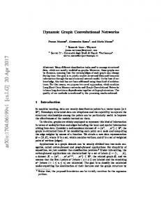
Random Graph Ensemble
Predictive Modeling
G-CNN Features
Softmax Output
G-CNN Population graph
Consensus
Class Label
Features
G-CNN N-dimensional feature per node
Features
Figure 2: An overview of the proposed approach for predictive modeling with non-imaging features encoded as a population graph and imaging features defined as functions on the nodes. We construct a randomized ensemble of population graphs, employ graph CNNs to build models and utilize a consensus strategy to perform the actual classification.
tics. Second, graph CNNs provide a powerful computing framework to make inferences on graphs, by treating the subject-specific image features as a function, f : V 7→ RN , defined at the nodes of the population graph. In addition to existing population graph construction strategies, we study the use of graph kernel similarities obtained by treating the measurements for each subject as a graph representation. Note, the latter is a subject-specific graph and can effectively model the spatio-temporal statistics of the brain activity. Our results show that the proposed bootstrapped G-CNN approach achieves the state-of-the-art performance in ASD classification and more interestingly, the graph ensemble strategy improves the prediction accuracies of all population graph construction approaches. In addition, the proposed bootstrapping reduces the sensitivity of the prediction performance to the graph construction step. Consequently, even non-experts can design simpler graphs, which, with bootstrapping, can perform on par with more sophisticated graph construction strategies.
2. Proposed Approach Figure 2 illustrates an overview of the proposed approach for predictive modeling in ASD classification. As it can be observed, the pipeline requires an initial population graph and the features at each node (i.e. subject) in the graph as inputs. Subsequently, we create an ensemble of randomized graph realizations and invoke the training of a graph CNN model for every realization. The output layer of these neural networks implement the softmax function, which computes the probabilities for class association of each node. Finally, the consensus module fuses the decisions from the ensemble to obtain the final class label. 3
In this section, we begin describing the proposed approach for predictive modeling to classify subjects with autism. More specifically, we describe the feature extraction procedure and the different strategies adopted for constructing population graphs. In the next section, we will present the predictive modeling algorithm, based on graph CNNs, that incorporates both the extracted features and information from the population graph. 2.1 Feature Extraction: The Connectivity Matrix Feature design has become an integral part of advanced machine learning systems. A good feature representation is characterized by its ability to describe the variabilities in the dataset, while being concise and preferably low-dimensional. It has been recently shown in Abraham et al. (2017) that the connectivity matrix can be reliably estimated from the resting state fMRI data as the covariance matrix obtained using the Ledoit-Wolf shrinkage estimator. Denoting the total number of regions of interest for each subject as d, the resulting d×d covariance matrix captures the relationships between the time-series measurements from the different ROIs. As shown in Abraham et al. (2017), these features are informative and can be directly used for classification by using the vectorized upper triangular part of the covariance matrix as the feature for each subject. Though more sophisticated feature learning strategies could be employed, we observed in our experiments that the connectivity matrix produces the best performance. Consequently, we adopt that feature representation in our approach. Since the resulting feature vector, commonly referred as the cursed representation, is high-dimensional, we perform dimensionality reduction on the features before using them to train a classifier. 2.2 Population Graph Construction Though the classifier can be directly trained using the extracted features, such an approach can fail to incorporate non-imaging/sensing information that can be critical to discriminate between different classes. For example, it is likely that there is discrepancy in some aspects of data collection at different sites, or the gender of the subject is important in generalizing autism spectrum disorder classifiers. It is non-trivial to directly incorporate such information into the subject features, but a graph can be a very intuitive way to introduce these relationships into the learning process. Graphs are natural data structures to model data in high dimensional spaces, where nodes represent the subjects and the edges describe the relations between them. This can be particularly effective while studying larger populations for traits of interest, because the graph can encode information that is different from the imaging features estimated for each subject independently. Furthermore, this can provide additional context to the machine learning algorithm used for prediction, thereby avoiding overfitting in cases of limited training data. It is important to distinguish the population graph construction process from graphs that are used to analyze the brain activity of each subject, i.e. connectivity matrix of statistical dependencies between different ROIs. Common data processing tasks such as filtering and localized transforms of signals do not directly generalize to irregular domains such as signals defined on graphs. Consequently, several graph signal processing tools have been developed to generalize ideas from Euclidean domain analysis. In particular, spectral filtering and wavelet analysis have become popular graph signal processing techniques in several applications Shuman et al. (2013). These 4
ideas have been further extended to build convolutional neural networks directly in the graph domain, which take advantage of the fact that convolutions are multiplications in the spectral domain (Defferrard et al. (2016); Kipf and Welling (2017)). In this paper, we propose to use graph convolutional neural networks (G-CNNs) to address the task of ASD classification using a population graph, with each node being characterized by the extracted features. An inherent challenge with such an analysis is that the results obtained are directly dictated by the weighted graph defined for the analysis. Consequently, designing suitable weighted graphs that capture the geometric structure of data is essential for meaningful analysis. In our context, the population graph construction determines how two subjects are connected, so that context information could be shared between them. In addition to approaches that employ simple heuristics (e.g. distances between features) or domain-specific characteristics (e.g. gender), we also investigate the use of a more sophisticated graph construction strategy, aimed at exploiting the spatio-temporal statistics of each subject. Here is the list of graph construction mechanisms adopted in this paper: • Site and Gender: Previous studies have showed that the geographical site information and the gender of the subject are important to build generalizable models and hence we use them to define the similarity graph between subjects. If two subjects have the same gender, they are given a score of ssex = λ1 > 1, and 1 if they are not. Similarity, the subjects were given a score of ssite = λ2 > 1, if they were processed at the same site, and 1 if not. • Linear Kernel Feature Graph: The edge weights of the graph are computed as the Euclidean dot product or a linear kernel, between connectivity features from two different ROIs, for a given subject. As expected, this graph does not provide any additional information because it is directly based on the features that were defined at the nodes. However, the authors in Parisot et al. (2017) showed that this can be combined with the gender and site graphs to build a new graph with additional information for improved prediction. • Graph Kernel on the Connectivity Matrix: This graph is constructed by interpreting the connectivity matrix as an adjacency matrix of a graph. We refer to this as the subject graph. This has favorable properties in that it can model the spatiotemporal statistics between ROIs explicitly as opposed to vectorizing them. This is followed by defining a graph kernel such as Weisfeler-Lehman (Shervashidze et al. (2011)) on pairs of subject graphs, resulting in a kernel matrix that can be used for classification or prediction Jie et al. (2014). In contrast, we interpret the resulting similarity kernel matrix as the population graph, after multiplying them edge weights from the gender and site graphs.
3. Predictive Modeling: Randomized Ensemble of G-CNNs In this section we briefly introduce convolutional neural networks on graphs, and present our bootstrapped training strategy using an ensemble of randomized population graphs. 5
3.1 Graph Convolutional Neural Networks Convolutional neural networks enable extraction of statistical features from structured data, in the form of local stationary patterns, and their aggregation for different semantic analysis tasks, e.g. image recognition or activity analysis. When the signal of interest does not lie on a regular domain, for example graphs, generalizing CNNs is particuarly challenging due to the presence of convolution and pooling operators, typically defined on regular grids. In graph signal processing theory, this challenge is alleviated by switching to the spectral domain, where the convolution operations can be viewed as simple multiplications. In general, there exists no mathematical definition for the translation operation on graphs. However, a spectral domain approach defines the localization operator on graphs via convolution with a Kronecker delta signal. However, localizing a filter in the spectral domain requires the computation of the graph Fourier transform and hence translations on graphs are computationally expensive. Before we describe the graph CNN architecture used in our approach, we define the Fourier transform for signals on graphs. Preliminaries: Formally, an undirected weighted graph is represented by G = (V, E, W), where V denotes the set of vertices or nodes, E denotes the set of edges and W is the adjacency matrix that specifies the weights between edges Wij , ∀ei , ej ∈ E. The fundamental component of graph analysis isPthe normalized graph Laplacian L, which is defined as I − D−1/2 WD−1/2 , where Dii = j Wij is the degree matrix and I denotes the identity matrix. The set of eigenvectors of the Laplacian are referred to as the graph Fourier basis, L = UΛUT , and hence the Fourier transform of a signal x ∈ RN is defined as UT x. Finally, the spectral filtering operation can be defined as y = gθ (L)x = Ugθ (Λ)UT x, where gθ is the parametric filter. Formulation: Since spectral filtering is computationally prohibitive as the number of nodes in the graph increases, Hammond et al. (2011) proposed to approximate gθ (Λ) as a truncated expansion in terms of the Chebyshev polynomials recursively.
gθˆ(Λ) ≈
K X
˜ θˆk Tk (Λ),
(1)
k=0
˜ where θˆ is the set of Chebyshev coefficients, K is the order for the approximation, Λ are rescaled eigenvalues and the Chebyshev polyomials Tk (x) are recursively defined as 2xTk−1 (x) − Tk−2 (x). Using this approximation in the spectral filtering operation implies that the filtering is K−localized, i.e., the filtering depends only on the K neighborhood nodes. We can use this K-localized filtering to define convolutional neural networks on graphs. For example, the approach in Kipf and Welling (2017) uses K = 1 such that the layerwise computation is linear w.r.t L. Though, this is a crude approximation, by stacking multiple layers one can still recover a large class of complex filter functions, that are not just limited to the linear functions supported by the first order Chebyshev approximation. The resulting filtering can then be expressed as gθˆ ? x = θˆ0 x − θˆ1 D−1/2 WD−1/2 x. 6
(2)
Here, ? indicates the convolution operation in the spatial domain. Note that, the filter parameters are shared over the whole graph. In summary, the complete processing in a layer is defined as follows: Given an input function X ∈ RT ×N , where T is the number of nodes, and N is the dimension of the multivariate function at each node, the activations can be computed as ˜ −1/2 W ˜D ˜ −1/2 XΘ). σ(D
(3)
Here Θ ∈ RN ×F is the set of filter parameters, the graph Laplacian is reparameterized as ˜ −1/2 W ˜D ˜ −1/2 = I + D−1/2 WD−1/2 . The activation function σ is chosen to be ReLU in D our implementation. This linear formulation of graph convolutional networks is much more computationally efficient compared to the accurate filtering implementation. 3.2 Ensemble Learning As described in the previous section, population graphs provide a convenient way to incorporate non-imaging features into the predictive modeling framework, where the connectivity features from fMRI data are used as a function on the graph. While G-CNN can automatically infer spectral filters for achieving discrimination across different classes, the sensitivity of its performance to the choice of the population graph is not straightforward to understand. Consequently, debugging and fine-tuning these networks can be quite challenging. The conventional approach to building robust predictive models is to infer an ensemble of weak learners from data and then fuse the decisions using a consensus strategy. The need for ensemble models in supervised learning has been well-studied Dietterich (2000). A variety of bootstrapping techniques have been developed, wherein multiple weak models are inferred using different random subsets of data. The intuition behind the success of this approach is statistical, whereby different models may have a similar training error when learned using a subset of training samples, but their performance on test data can be different since they optimize for different regions of the input data space. We employ a similar intuition to building models with population graphs, wherein the quality of different similarity metrics for graph construction can lead to vastly different predictive models. More specifically, starting with a population graph, we create an ensemble of graphs, {Gp }Pp=1 , by dropping out a pre-defined factor of edges randomly. In this paper, we use a uniform random distribution for the dropout, though more sophisticated weighted distributions could be used. For each of the graphs in the ensemble, we build a G-CNN model (details in Section 4) with the connectivity features as the N −dimensional multivariate function at each node. The output of each of the networks is a softmax function for each node, indicating the probability for the subject to be affected by ASD. Note that, unlike conventional ensemble learners, we do not subsample data, but only subsample edges of the population graph. Given the decisions from all the weak learners, we employ simple consensus strategies such as averaging or obtaining the maximum of the probabilities estimated by each of the G-CNNs for a test subject. As we will show in our experimental results with the ABIDE dataset, the proposed ensemble approach boosts the performance of all the population graph construction strategies discussed in Section 2. 7
4. Experiments In this section, we describe our experiments to evaluate the performance of the proposed ensemble approach in ASD classification, for different population graphs. For comparison, we report the state-of-the-art results obtained using the methods in Abraham et al. (2017) and Parisot et al. (2017). 4.1 The ABIDE dataset We present our results on the Autism Brain Imaging Data Exchange (ABIDE) dataset Di Martino et al. (2014) that contains resting state fMRI data (rs-fMRI) for 1112 patients, as part of the preprocessed connectomes project 2 . The pre-processing includes slice-timing correction, motion correction, and intensity normalization, depending on the pipeline used. We follow the same preprocessing pipeline (C-PAC) and atlases (Harvard-Oxford) as described in Abraham et al. (2017), in order to facilitate easy comparison – this resulted in a dataset with 872 of the initial 1112 patients available, from 20 different sites. The task is now to diagnose a patient as being of two classes – Autism Spectrum Disorder (ASD) or Typical Control (TC). These labels are available separately 3 . The resulting data per subject consists of the mean time series obtained from the rsfMRI for each Region of Interest (ROI). In total, there are 111 ROIs for the HO atlas considered here, resulting in the data, for the ith subject, of size R111×T matrix, where T is the total number of slices in the fMRI measurement. We use the same train/test splits as Abraham et al. (2017) and the 10-fold split of the ABIDE dataset, resulted in 696 patients used for training and the remaining 175 patients for testing. Instead of reporting the average performance, we report the accuracies for the best performing and the worst performing splits chosen w.r.t the baseline described in the next subsection (i.e split 1, split 8), since this provides a much better understanding of the performance variabilities. 4.2 Methods Baseline: First, for each patient we estimate the connectivity matrix between the ROIs, as the covariance of the multivariate time-series data estimated using the Ledoit-Wolf shrinkage estimator. In order to establish a baseline, we construct the connectivity feature by vectorizing the upper triangular part of the covariance matrix and performing dimensionality reduction (60D) on the vectorized feature. The connectivity features of the subjects are then fed into a linear SVM Abraham et al. (2017) and a kernel SVM with the radial basis function kernel. Graph Convolutional Neural Network (G-CNN): We use the G-CNN implementation from Kipf and Welling (2017), particularly the Chebychev polynomial approximation for the Fourier basis as described in Defferrard et al. (2016). We constructed a fully convolutional network, with 6 layers of 64 neurons each, a learning rate of 0.005, and dropout of 0.1/0.2 depending on the graph. We used Chebychev polynomials upto degree 3 to approximate the Graph Fourier Transform in the G-CNN in all our experiments. The G-CNN requires a 2. http://preprocessed-connectomes-project.org/abide/ 3. Column named DX GROUP in https://s3.amazonaws.com/fcp-indi/data/Projects/ABIDE_ Initiative/Phenotypic_V1_0b_preprocessed1.csv
8
Population Graph Gsex, site
GLinear Kernel
GGraph Kernel
Predictive Model Linear SVM (baseline) Kernel SVM (baseline) G-CNN Ensemble G-CNN (avg) Ensemble G-CNN (max) G-CNN Ensemble G-CNN (avg) Ensemble G-CNN (max) G-CNN Ensemble G-CNN (avg) Ensemble G-CNN (max)
Best Split (%) 66.28 69.14 64.00 67.42 68.57 69.14 69.14 69.14 66.27 69.14 70.28
Worst Split(%) 65.14 62.29 62.87 68.00 67.42 64.57 65.14 66.28 65.71 67.42 66.28
Table 1: Classification Accuracy for the ABIDE dataset (Di Martino et al. (2014)) using the proposed approach. For comparison, we report the state-of-the-art results obtained using linear SVM Abraham et al. (2017) and linear kernel graphs Parisot et al. (2017). In all the cases, using the proposed Random Graph Ensemble approach leads to 1 − 6% percentage points improvement in accuracy. The results for the ensemble case were obtained using an ensemble of 5 random graphs.
suitable graph G, features defined for each node, and the classification label y ∈ {0, 1} for the binary classification task. For a given graph, the best results were obtained typically in around 100 − 150 epochs, similar numbers have also been reported in Parisot et al. (2017). Ensemble G-CNN: For a given graph G, we generate P new graphs such that the new set of graphs {G0 , G1 . . . GP } were obtained by randomly dropping 30 − 40% of the edges of G. The G-CNN for each graph was trained for 100 epochs, with a dropout of 0.1. The predictions from each model obtained using the ensemble are fused using two simple strategies - (a) avg, where we take the mean of the predictions and assign the class as the one with the largest value, (b) max, where we take the most confident value for each class and assign the label which has a higher value. In general, we found that a G-CNN for the ABIDE dataset, that is particularly sensitive, tends to overfit very easily making it extremely challenging to tune the hyperparameters. However, introducing randomness in the graphs significantly improved robustness and led to improved training, behaving a lot like dropout inside traditional neural networks. This behavior can be possibly attributed to the fact that the dropout in the G-CNN tends to ignore random edges in the hidden layers of the neural network, while we are proposing to use multiple randomized graphs in the input layer. In general, the random ensembles behave as weak learners, where the performance for each individual network is suboptimal, but the consensus decision is better than the state-of-the-art. 4.3 Classification Results The classification accuracy for different graphs and their corresponding random ensembles are shown in table 1. A few observations are important to note – There is a clear and 9
obvious advantage in using the graph based approach to classifying populations. This is especially true in datasets where the features alone are not sufficient, but require contextual information, which a population graph can provide. Secondly, the difference in performance for different graphs illustrates the importance of graph construction, further emphasizing the need for robust training strategies such as those proposed in this paper. It is also seen that using a random graph ensemble significantly improves performance by up to 6% higher than the state-of-the-art using only features as in Abraham et al. (2017). We also show improvements over using the linear kernel graph proposed in a recent manuscript (Parisot et al. (2017)). Finally, it can be observed that the best performing split has a consistently high performance across different kinds of graphs and only marginally better than the baseline, perhaps indicating that the connectivity features dictate the performance in that case. In contrast, the worst performing split contains nearly 6% lower performance without using the graph information. We observe that the largest gains in performance are in this split, indicating that the proposed ensemble strategy is able to recover important information for classification, which can be missed by heuristic graph construction. Another interesting observation is that a simple domain-specific graph such as the Gsex, site , can perform as well as any state-of-the-art method, when couple with the proposed ensemble strategy.
5. Discussion and Future Work
In this paper we presented a training strategy for graph convolutional neural networks (GCNNs), that have been recently proposed as a promising solution to the node classification problem in graph structured data. We focused particularly on autism spectrum disorder classification using time series extracted from resting state fMRI. The problem is challenging because each subject contains time series data from multiple regions of interest in the brain. A population graph, in addition to the imaging features, can provide more contextual information, leading to better classification performance. However, the consequence of building a population graph is that it becomes an important step in the process, and graph construction is hard in general, because it is hard to know beforehand which relationships are actually important to the prediction task. To circumvent this challenge, we propose to use bootstrapping as a way to reduce the sensitivity of the initial graph construction step, by generating multiple random graphs from the initial population graph. We train a G-CNN for each randomized graph, and fuse their predictions at the end, based on simple consensus strategies. These individual predictive models behave as weak learners, that can be aggregated to produce superior classification performance. The proposed work opens several new avenues of future work including (a) pursuing a theoretical justification behind the improved performance from randomized ensembles, (b) extending these ideas by using an ensemble of random binary graphs, with appropriate probability distributions, which are very cheap to construct, and (c) performing fusion in the hidden layers instead of final layer, which involves training the ensemble of networks together. 10
References Alexandre Abraham, Michael P Milham, Adriana Di Martino, R Cameron Craddock, Dimitris Samaras, Bertrand Thirion, and Gael Varoquaux. Deriving reproducible biomarkers from multi-site resting-state data: An autism-based example. NeuroImage, 147:736–745, 2017. Yashar Behzadi, Khaled Restom, Joy Liau, and Thomas T Liu. A component based noise correction method (compcor) for bold and perfusion based fmri. NeuroImage, 37 1:90–101, 2007. V.D. Calhoun, T. Adali, G.D. Pearlson, and J.J. Pekar. A method for making group inferences from functional mri data using independent component analysis. Human Brain Mapping, 14(3). Gang Chen, B. Douglas Ward, Chunming Xie, Wenjun Li, Zhilin Wu, Jennifer L. Jones, Malgorzata Franczak, Piero Antuono, and Shi-Jiang Li. Classification of alzheimer disease, mild cognitive impairment, and normal cognitive status with large-scale network analysis based on resting-state functional mr imaging. Radiology, 259(1):213–221, 2011. Micha¨el Defferrard, Xavier Bresson, and Pierre Vandergheynst. Convolutional neural networks on graphs with fast localized spectral filtering. In Advances in Neural Information Processing SystemsNIPS, pages 3837–3845, 2016. Adriana Di Martino, Chao-Gan Yan, Qingyang Li, Erin Denio, Francisco X Castellanos, Kaat Alaerts, Jeffrey S Anderson, Michal Assaf, Susan Y Bookheimer, Mirella Dapretto, et al. The autism brain imaging data exchange: towards a large-scale evaluation of the intrinsic brain architecture in autism. Molecular psychiatry, 19(6):659–667, 2014. Thomas G. Dietterich. Ensemble methods in machine learning. In Proceedings of the First International Workshop on Multiple Classifier Systems, MCS ’00, 2000. David K. Hammond, Pierre Vandergheynst, and Rmi Gribonval. Wavelets on graphs via spectral graph theory. Applied and Computational Harmonic Analysis, 30(2):129 – 150, 2011. Biao Jie, Daoqiang Zhang, Chong-Yaw Wee, and Dinggang Shen. Topological graph kernel on multiple thresholded functional connectivity networks for mild cognitive impairment classification. Human brain mapping, 35(7):2876–2897, 2014. A. M. Clare Kelly, Lucina Q. Uddin, Bharat B. Biswal, F. Xavier Castellanos, and Michael P. Milham. Competition between functional brain networks mediates behavioral variability. NeuroImage, 39(1):527–527, January 2008. Thomas N Kipf and Max Welling. Semi-supervised classification with graph convolutional networks. In International Conference on Learning Representations (ICLR, 2017. Sarah Parisot, Sofia Ira Ktena, Enzo Ferrante, Matthew Lee, Ricardo Guerrerro Moreno, Ben Glocker, and Daniel Rueckert. Spectral graph convolutions on population graphs for disease prediction. arXiv preprint arXiv:1703.03020, 2017. 11
Mark Plitt, Kelly Anne Barnes, and Alex Martin. Functional connectivity classification of autism identifies highly predictive brain features but falls short of biomarker standards. NeuroImage: Clinical, 7:359 – 366, 2015. Nino Shervashidze, Pascal Schweitzer, Erik Jan van Leeuwen, Kurt Mehlhorn, and Karsten M Borgwardt. Weisfeiler-lehman graph kernels. Journal of Machine Learning Research, 12(Sep):2539–2561, 2011. David I Shuman, Sunil K Narang, Pascal Frossard, Antonio Ortega, and Pierre Vandergheynst. The emerging field of signal processing on graphs: Extending highdimensional data analysis to networks and other irregular domains. IEEE Signal Processing Magazine, 30(3):83–98, 2013.
12