Crystal Graph Convolutional Neural Networks for an ... - Tian Xie

PHYSICAL REVIEW LETTERS 120, 145301 (2018)

Crystal Graph Convolutional Neural Networks for an Accurate and Interpretable Prediction of Material Properties Tian Xie and Jeffrey C. Grossman Department of Materials Science and Engineering, Massachusetts Institute of Technology, Cambridge, Massachusetts 02139, USA (Received 18 October 2017; revised manuscript received 15 December 2017; published 6 April 2018) The use of machine learning methods for accelerating the design of crystalline materials usually requires manually constructed feature vectors or complex transformation of atom coordinates to input the crystal structure, which either constrains the model to certain crystal types or makes it difficult to provide chemical insights. Here, we develop a crystal graph convolutional neural networks framework to directly learn material properties from the connection of atoms in the crystal, providing a universal and interpretable representation of crystalline materials. Our method provides a highly accurate prediction of density functional theory calculated properties for eight different properties of crystals with various structure types and compositions after being trained with 104 data points. Further, our framework is interpretable because one can extract the contributions from local chemical environments to global properties. Using an example of perovskites, we show how this information can be utilized to discover empirical rules for materials design. DOI: 10.1103/PhysRevLett.120.145301

Machine learning (ML) methods are becoming increasingly popular in accelerating the design of new materials by predicting material properties with accuracy close to ab initio calculations, but with computational speeds orders of magnitude faster [1–3]. The arbitrary size of crystal systems poses a challenge as they need to be represented as a fixed length vector in order to be compatible with most ML algorithms. This problem is usually resolved by manually constructing fixed length feature vectors using simple material properties [1,3–6] or designing symmetry-invariant transformations of atom coordinates [7–9]. However, the former requires a case-by-case design for predicting different properties, and the latter makes it hard to interpret the models as a result of the complex transformations. In this Letter, we present a generalized crystal graph convolutional neural networks (CGCNN) framework for representing periodic crystal systems that provides both material property prediction with density functional theory (DFT) accuracy and atomic level chemical insights. Recent advances in “deep learning” have enabled learning from a very raw representation of data, e.g., pixels of an image, making it possible to build general models that outperform traditionally expert designed representations [10]. By looking into the simplest form of crystal representation, i.e., the connection of atoms in the crystal, we directly build convolutional neural networks on top of crystal graphs generated from crystal structures. The CGCNN achieves similar accuracy with respect to DFT calculations as DFT compared with experimental data for eight different properties after being trained with data from the Materials Project [11], indicating the generality of this method. We also 0031-9007=18=120(14)=145301(6)

demonstrate the interpretability of the CGCNN by extracting the energy of each site in the perovskite structure from the total energy, an example of learning the contribution of local chemical environments to the global property. The empirical rules generalized from the results are consistent with the common knowledge for discovering more stable perovskites and can significantly reduce the search space for high throughput screening. The main idea in our approach is to represent the crystal structure by a crystal graph that encodes both atomic information and bonding interactions between atoms, and then build a convolutional neural network on top of the graph to automatically extract representations that are optimum for predicting target properties by training with DFT calculated data. As illustrated in Fig. 1(a), a crystal graph G is an undirected multigraph which is defined by nodes representing atoms and edges representing connections between atoms in a crystal (the method for determining atom connectivity is explained in the Supplemental Material [12]). The crystal graph is unlike normal graphs since it allows multiple edges between the same pair of end nodes, a characteristic for crystal graphs due to their periodicity, in contrast to molecular graphs. Each node i is represented by a feature vector vi, encoding the property of the atom corresponding to node i. Similarly, each edge ði; jÞk is represented by a feature vector uði;jÞk corresponding to the kth bond connecting atom i and atom j. The convolutional neural networks built on top of the crystal graph consist of two major components: convolutional layers and pooling layers. Similar architectures have been used for computer vision [22], natural language

145301-1

© 2018 American Physical Society

PHYSICAL REVIEW LETTERS 120, 145301 (2018) property y, defined by a cost function Jðy; yˆ Þ. The whole CGCNN can be considered as a function f parametrized by weights W that maps a crystal C to the target property yˆ . Using backpropagation and stochastic gradient descent (SGD), we can solve the following optimization problem by iteratively updating the weights with DFT calculated data: minJ(y; fðC; WÞ) W

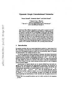
FIG. 1. Illustration of the crystal graph convolutional neural networks. (a) Construction of the crystal graph. Crystals are converted to graphs with nodes representing atoms in the unit cell and edges representing atom connections. Nodes and edges are characterized by vectors corresponding to the atoms and bonds in the crystal, respectively. (b) Structure of the convolutional neural network on top of the crystal graph. R convolutional layers and L1 hidden layers are built on top of each node, resulting in a new graph with each node representing the local environment of each atom. After pooling, a vector representing the entire crystal is connected to L2 hidden layers, followed by the output layer to provide the prediction.

processing [23], molecular fingerprinting [24] and general graph-structured data [25,26], but not for crystal property prediction to the best of our knowledge. The convolutional layers iteratively update the atom feature vector vi by “convolution” with surrounding atoms and bonds with a nonlinear graph convolution function,
 ðtþ1Þ ðtÞ ðtÞ vi ¼ Conv vi ; vj ; uði;jÞk ; ði; jÞk ∈ G: ð1Þ After R convolutions, the network automatically learns the ðRÞ feature vector vi for each atom by iteratively including its surrounding environment. The pooling layer is then used for producing an overall feature vector vc for the crystal, which can be represented by a pooling function, ð0Þ

ð0Þ

ð0Þ

ðRÞ

vc ¼ Poolðv0 ; v1 ; …; vN ; …; vN Þ

ð2Þ

that satisfies permutational invariance with respect to atom indexing and size invariance with respect to unit cell choice. In this work, a normalized summation is used as the pooling function for simplicity, but other functions can also be used. In addition to the convolutional and pooling layers, two fully connected hidden layers with the depths of L1 and L2 are added to capture the complex mapping between crystal structure and property. Finally, an output layer is used to connect the L2 hidden layer to predict the target property yˆ. The training is performed by minimizing the difference between the predicted property yˆ and the DFT calculated

ð3Þ

the learned weights can then be used to predict material properties and provide chemical insights for future materials design. In the Supplemental Material (SM) [12], we use a simple example to illustrate how a CGCNN composed of one linear convolution layer and one pooling layer can differentiate two crystal structures. With multiple convolution layers, pooling layers, and hidden layers, the CGCNN can extract any structure differences based on the atom connections and discover the underlaying relations between structure and property. To demonstrate the generality of the CGCNN, we train the model using calculated properties from the Materials Project [11]. We focus on two types of generality in this work: (1) the structure types and chemical compositions for which our model can be applied and (2) the number of properties that our model can accurately predict. The database we used includes a diverse set of inorganic crystals ranging from simple metals to complex minerals. After removing ill-converged crystals, the full database has 46 744 materials covering 87 elements, 7 lattice systems, and 216 space groups. As shown in Fig. 2(a), the materials consist of as many as seven different elements, with 90% of them binary, ternary, and quaternary compounds. The number of atoms in the primitive cell ranges from 1 to 200, and 90% of crystals have less than 60 atoms (Fig. S2). Considering most of the crystals originate from the Inorganic Crystal Structure Database [27], this database is a good representation of known stoichiometric inorganic crystals. The CGCNN is a flexible framework that allows variance in the crystal graph representation, neural network architecture, and training process, resulting in different f in Eq. (3) and prediction performance. To choose the best model, we apply a train-validation scheme to optimize the prediction of formation energies of crystals. Each model is trained with 60% of the data and then validated with 20% of the data, and the best-performing model in the validation set is selected. In our study, we find that the neural network architecture, especially the form of convolution function in Eq. (1), has the largest impact on prediction performance. We start with a simple convolution function, ðtþ1Þ vi ¼g

145301-2

  X ðtÞ ðtÞ ðtÞ ðtÞ ðtÞ vj ⊕ uði;jÞk W c þ vi W s þ b ; j;k

ð4Þ

PHYSICAL REVIEW LETTERS 120, 145301 (2018) (a)

(b)

(c)

(d)

FIG. 2. Performance of CGCNN on the Materials Project database [11]. (a) Histogram representing the distribution of the number of elements in each crystal. (b) Mean absolute error as a function of training crystals for predicting formation energy per atom using different convolution functions. The shaded area denotes the MAEs of DFT calculations compared with experiments [28]. (c) 2D histogram representing the predicted formation per atom against DFT calculated value. (d) Receiver operating characteristic curve visualizing the result of metalsemiconductor classification. It plots the proportion of correctly identified metals (true positive rate) against the proportion of wrongly identified semiconductors (false positive rate) under different thresholds.

where ⊕ denotes concatenation of atom and bond feature ðtÞ ðtÞ vectors, W c , W s , and bðtÞ are the convolution weight matrix, self-weight matrix, and bias of the tth layer, respectively, and g is the activation function for introducing nonlinear coupling between layers. By optimizing hyperparameters in Table S1, the lowest mean absolute error (MAE) for the validation set is 0.108 eV=atom. One limitation of Eq. (4) is that it uses a shared convolution ðtÞ weight matrix W c for all neighbors of i, which neglects the differences of interaction strength between neighbors. To overcome this problem, we design a new convolution function that first concatenates neighbor vectors ðtÞ ðtÞ ðtÞ zði;jÞ ¼ vi ⊕ vj ⊕ uði;jÞk , then perform convolution by k

ðtþ1Þ

vi

ðtÞ

¼ vi þ ⊙g




 X
ðtÞ ðtÞ ðtÞ σ zði;jÞ W f þ bf j;k

ðtÞ ðtÞ zði;jÞ W s k

function, a significant improvement compared to Eq. (4). In Fig. S3, we compare the effects of several other hyperparameters on the MAE which are much smaller than the effect of the convolution function. Figures 2(b) and 2(c) show the performance of the two models on 9350 test crystals for predicting the formation energy per atom. We find a systematic decrease of the MAE of the predicted values compared with DFT calculated values for both convolution functions as the number of training data is increased. The best MAEs we achieved with Eqs. (4) and (5) are 0.136 and 0.039 eV=atom, respectively, and 90% of the crystals are predicted within 0.3 and 0.08 eV=atom errors. In comparison, Kirklin et al. reports that the MAE of the DFT calculation with respect to experimental measurements in the Open Quantum Materials Database is 0.081–0.136 eV=atom depending on whether the energies of the elemental reference states are fitted, although they also find a large MAE of 0.082 eV=atom between different sources of experimental data. Given the comparison, our CGCNN approach provides a reliable estimation of DFT calculations and can potentially be applied to predict properties calculated by more accurate methods like GW [30] and quantum Monte Carlo calculations [31]. After establishing the generality of the CGCNN with respect to the diversity of crystals, we next explore its prediction performance for different material properties. We apply the same framework to predict the absolute energy, band gap, Fermi energy, bulk moduli, shear moduli, and Poisson ratio of crystals using DFT calculated data from the Materials Project [11]. The prediction performance of Eq. (5) is improved compared to Eq. (4) for all six properties (Table S4). We summarize the performance in Table I and the corresponding 2D histograms in Fig. S4. As we can see, the MAEs of our model are close to or higher than DFT accuracy relative to experiments for most properties when ∼104 training data are used. For elastic properties, the errors are higher since less data are available, and the accuracy of DFT relative to experiments can be expected if ∼104 training data are available (Fig. S5). TABLE I. Summary of the prediction performance of seven different properties on test sets.

k

þ

ðtÞ bs



Property

;

ð5Þ

where ⊙ denotes element-wise multiplication and σ denotes a sigmoid function. In Eq. (5), the σð·Þ functions as a learned weight matrix to differentiate interactions ðtÞ between neighbors and adding vi makes learning deeper networks easier [29]. We achieve MAE on the validation set of 0.039 eV=atom using the modified convolution

Formation energy Absolute energy Band gap Fermi energy Bulk moduli Shear moduli Poisson ratio

145301-3

# of train data

Unit MAEmodel

MAEDFT

28 046

eV=atom 0.039 0.081–0.136 [28]

28 046

eV=atom 0.072

16 458 28 046 2041 2041 2041

eV eV log(GPa) log(GPa) 



0.388 0.6 [32] 0.363  0.054 0.050 [13] 0.087 0.069 [13] 0.030 

PHYSICAL REVIEW LETTERS 120, 145301 (2018) Recently, Jong et al. [33] developed a statistical learning (SL) framework using multivariate local regression on crystal descriptors to predict elastic properties using the same data from the Materials Project. By using the same number of training data, our model achieves root mean squared error (RMSE) on test sets of 0.105 log(GPa) and 0.127 log(GPa) for the bulk and shear moduli, which is similar to the RMSE of SL on the entire data set of 0.0750 log(GPa) and 0.1378 log(GPa). Comparing the two methods, the CGCNN predicts properties by extracting features only from the crystal structure, while SL depends on crystal descriptors like cohesive energy and volume per atom. Recently, 1585 new crystals with elastic properties have been uploaded to the Materials Project database. Our model in Table I achieves MAE of 0.077 log(GPa) for bulk moduli and 0.114 log(GPa) for shear moduli on these crystals, showing good generalization to materials from potentially different crystal groups. In addition to predicting continuous properties, the CGCNN can also predict discrete properties by changing the output layer. By using a softmax activation function for the output layer and a cross entropy cost function, we can predict the classifications of metal and semiconductor with the same framework. In Fig. 2(d), we show the receiver operating characteristic curve of the prediction on 9350 test crystals. Excellent prediction performance is achieved with the area under the curve at 0.95. By choosing a threshold of 0.5, we get metal prediction accuracy at 0.80, semiconductor prediction accuracy at 0.95, and overall prediction accuracy at 0.90. Model interpretability is a desired property for any ML algorithm applied in materials science, because it can provide additional information for material design which may be more valuable than simply screening a large number of materials. However, nonlinear functions are needed to learn the complex structure-property relations, resulting in ML models that are difficult to interpret. The CGCNN resolves this dilemma by separating the convolution and pooling layers. After the R convolutional and L1 hidden layers, we ðRÞ map the last atom feature vector vi to a scalar v˜ i and perform a linear pooling to predict the target property directly without the L2 hidden layers (details discussed in SM [12]). Therefore, we can learn the contribution of different local chemical environments, represented by v˜ i for each atom, to the target property while maintaining a model with high capacity to ensure the prediction performance. We demonstrate how this local chemical environment related information can be used to provide chemical insights and guide the material design by a specific example: learning the energy of each site in perovskites from the total energy above hull data. Perovskite is a crystal structure type with the form of ABX3 , where the site A atom sits at a corner position, the site B atom sits at a body centered position, and site X atoms sit at face centered positions [Fig. 3(a)]. The database [34] we use includes the energy above hull of 18 928 perovskite crystals, in which A and B sites can be any

(a)

(b)

(c)

(d)

FIG. 3. Extraction of site energy of perovskites from total formation energy. (a) Structure of perovskites. (b) 2D histogram representing the predicted total energy above hull against DFT calculated value. (c),(d) Periodic table with the color of each element representing the mean of the site energy when the element occupies A site (c) or B site (d).

nonradioactive metals and X sites can be one or several elements from O, N, S, and F. We use the CGCNN with a linear pooling to predict the total energy above hull of perovskites in the database, using Eq. (4) as the convolution function. The resulting MAE on 3787 test perovskites is 0.130 eV=atom as shown in Fig. 3(b), which is slightly higher than using a complete pooling layer and L2 hidden layers (0.099 eV=atom as shown in Fig. S6) due to the additional constraints introduced by the simplified pooling layer. However, this CGCNN allows us to learn the energy of each site in the crystal while training with the total energy above hull, providing additional insights for material design. Figures 3(c) and 3(d) visualize the mean of the predicted site energies when each element occupies the A and B site, respectively. The most stable elements that occupy the A site are those with large radii due to the space needed for 12 coordinations. In contrast, elements with small radii like Be, B, and Si are the most unstable for occupying the A site. For the B site, elements in groups 4, 5, and 6 are the most stable throughout the periodic table. This can be explained by crystal field theory, since the configuration of d electrons of these elements favors the octahedral coordination in the B site. Interestingly, the visualization shows that large atoms from groups 13–15 are stable in the A site, in addition to the well-known region of groups 1–3

145301-4

PHYSICAL REVIEW LETTERS 120, 145301 (2018) elements. Inspired by this result, we applied a combinatorial search for stable perovskites using elements from groups 13–15 as the A site and groups 4–6 as the B site. Because of the theoretical inaccuracies of DFT calculations and the possibility of metastable phases that can be stabilized by temperature, defects, and substrates, many synthesizable inorganic crystals have positive calculated energies above hull at 0 K. Some metastable nitrides can even have energies up to 0.2 eV=atom above hull as a result of the strong bonding interactions [35]. In this work, since some of the perovskites are also nitrides, we choose to set the cutoff energy for potential synthesizability at 0.2 eV=atom. We discovered 33 perovskites that fall within this threshold out of 378 in the entire data set, among which 8 are within the cutoff out of 58 in the test set (Table S5). Many of these compounds like PbTiO3 [36], PbZrO3 [36], SnTaO3 [37], and PbMoO3 [38] have been experimentally synthesized. Note that PbMoO3 has calculated energy of 0.18 eV=atom above hull, indicating that our choice of cutoff energy is reasonable. In general, chemical insights gained from the CGCNN can significantly reduce the search space for high throughput screening. In comparison, there are only 228 potentially synthesizable perovskites out of 18 928 in our database: the chemical insight increased the search efficiency by a factor of 7. In summary, the crystal graph convolutional neural networks present a flexible machine learning framework for material property prediction and design knowledge extraction. The framework provides a reliable estimation of DFT calculations using around 104 training data for eight properties of inorganic crystals with diverse structure types and compositions. As an example of knowledge extraction, we apply this approach to the design of new perovskite materials and show that information extracted from the model is consistent with common chemical insights and significantly reduces the search space for high throughput screening. The code for the CGCNN is available from Ref. [39]. This work was supported by Toyota Research Institute. Computational support was provided through the National Energy Research Scientific Computing Center, a DOE Office of Science User Facility supported by the Office of Science of the U.S. Department of Energy under Contract No. DE-AC02-05CH11231, and the Extreme Science and Engineering Discovery Environment, supported by National Science Foundation Grant No. ACI-1053575.

[1] A. Seko, A. Togo, H. Hayashi, K. Tsuda, L. Chaput, and I. Tanaka, Phys. Rev. Lett. 115, 205901 (2015). [2] F. A. Faber, A. Lindmaa, O. A. von Lilienfeld, and R. Armiento, Phys. Rev. Lett. 117, 135502 (2016). [3] D. Xue, P. V. Balachandran, J. Hogden, J. Theiler, D. Xue, and T. Lookman, Nat. Commun. 7, 11241 (2016). [4] O. Isayev, C. Oses, C. Toher, E. Gossett, S. Curtarolo, and A. Tropsha, Nat. Commun. 8, 15679 (2017).

[5] L. M. Ghiringhelli, J. Vybiral, S. V. Levchenko, C. Draxl, and M. Scheffler, Phys. Rev. Lett. 114, 105503 (2015). [6] O. Isayev, D. Fourches, E. N. Muratov, C. Oses, K. Rasch, A. Tropsha, and S. Curtarolo, Chem. Mater. 27, 735 (2015). [7] K. T. Schütt, H. Glawe, F. Brockherde, A. Sanna, K. R. Müller, and E. K. U. Gross, Phys. Rev. B 89, 205118 (2014). [8] F. Faber, A. Lindmaa, O. A. von Lilienfeld, and R. Armiento, Int. J. Quantum Chem. 115, 1094 (2015). [9] A. Seko, H. Hayashi, K. Nakayama, A. Takahashi, and I. Tanaka, Phys. Rev. B 95, 144110 (2017). [10] Y. LeCun, Y. Bengio, and G. Hinton, Nature (London) 521, 436 (2015). [11] A. Jain, S. P. Ong, G. Hautier, W. Chen, W. D. Richards, S. Dacek, S. Cholia, D. Gunter, D. Skinner, G. Ceder et al., APL Mater. 1, 011002 (2013). [12] See Supplemental Material at http://link.aps.org/ supplemental/10.1103/PhysRevLett.120.145301 for further details, which includes Refs. [4,13–21]. [13] M. De Jong, W. Chen, T. Angsten, A. Jain, R. Notestine, A. Gamst, M. Sluiter, C. K. Ande, S. Van Der Zwaag, J. J. Plata et al., Sci. Data 2, 150009 (2015). [14] R. Sanderson, Science 114, 670 (1951). [15] R. Sanderson, J. Am. Chem. Soc. 74, 4792 (1952). [16] B. Cordero, V. Gómez, A. E. Platero-Prats, M. Rev´es, J. Echeverría, E. Cremades, F. Barragán, and S. Alvarez, Dalton Trans. 21, 2832 (2008). [17] A. Kramida, Y. Ralchenko, J. Reader et al., Atomic Spectra Database (National Institute of Standards and Technology, Gaithersburg, MD, 2013). [18] W. M. Haynes, CRC Handbook of Chemistry and Physics (CRC Press, Boca Raton, FL, 2014). [19] D. Kingma and J. Ba, arXiv:1412.6980. [20] N. Srivastava, G. E. Hinton, A. Krizhevsky, I. Sutskever, and R. Salakhutdinov, J. Mach. Learn. Res. 15, 1929 (2014). [21] V. A. Blatov, Crystallography Reviews 10, 249 (2004). [22] A. Krizhevsky, I. Sutskever, and G. E. Hinton, in Advances in Neural Information Processing Systems (MIT Press, Cambridge, MA, 2012), pp. 1097–1105. [23] R. Collobert and J. Weston, in Proceedings of the 25th International Conference on Machine Learning (ACM, New York, 2008), pp. 160–167. [24] D. K. Duvenaud, D. Maclaurin, J. Iparraguirre, R. Bombarell, T. Hirzel, A. Aspuru-Guzik, and R. P. Adams, in Advances in Neural Information Processing Systems (MIT Press, Cambridge, MA, 2015), pp. 2224–2232. [25] M. Henaff, J. Bruna, and Y. LeCun, arXiv:1506.05163. [26] J. Gilmer, S. S. Schoenholz, P. F. Riley, O. Vinyals, and G. E. Dahl, Proceedings of the 34th International Conference on Machine Learning, 2017, http://proceedings.mlr.press/ v70/gilmer17a.html. [27] M. Hellenbrandt, Crystallography Reviews 10, 17 (2004). [28] S. Kirklin, J. E. Saal, B. Meredig, A. Thompson, J. W. Doak, M. Aykol, S. Rühl, and C. Wolverton, npj Comput. Mater. 1, 15010 (2015). [29] K. He, X. Zhang, S. Ren, and J. Sun, in Proceedings of the IEEE Conference on Computer Vision and Pattern Recognition (IEEE, New York, 2016), pp. 770–778. [30] M. S. Hybertsen and S. G. Louie, Phys. Rev. B 34, 5390 (1986).

145301-5

PHYSICAL REVIEW LETTERS 120, 145301 (2018) [31] W. Foulkes, L. Mitas, R. Needs, and G. Rajagopal, Rev. Mod. Phys. 73, 33 (2001). [32] A. Jain, G. Hautier, C. J. Moore, S. P. Ong, C. C. Fischer, T. Mueller, K. A. Persson, and G. Ceder, Comput. Mater. Sci. 50, 2295 (2011). [33] M. De Jong, W. Chen, R. Notestine, K. Persson, G. Ceder, A. Jain, M. Asta, and A. Gamst, Sci. Rep. 6, 34256 (2016). [34] I. E. Castelli, T. Olsen, S. Datta, D. D. Landis, S. Dahl, K. S. Thygesen, and K. W. Jacobsen, Energy Environ. Sci. 5, 5814 (2012).

[35] W. Sun, S. T. Dacek, S. P. Ong, G. Hautier, A. Jain, W. D. Richards, A. C. Gamst, K. A. Persson, and G. Ceder, Sci. Adv. 2, e1600225 (2016). [36] G. Shirane, K. Suzuki, and A. Takeda, J. Phys. Soc. Jpn. 7, 12 (1952). [37] J. Lang, C. Li, X. Wang et al., Mater. Today: Proc. 3, 424 (2016). [38] H. Takatsu, O. Hernandez, W. Yoshimune, C. Prestipino, T. Yamamoto, C. Tassel, Y. Kobayashi, D. Batuk, Y. Shibata, A. M. Abakumov et al., Phys. Rev. B 95, 155105 (2017). [39] CGCNN website, https://github.com/txie-93/cgcnn.

145301-6