Boundary conditions for matrix of variations in refractive waveguides ...

arXiv:1212.6068v1 [math-ph] 25 Dec 2012

Boundary conditions for matrix of variations in refractive waveguides with rough bottom I.P. Smirnov Institute of Applied Physics RAS, 46 Ul’yanova Street, Nizhny Novgorod, Russia Abstract The solution of the Helmholtz equation in optical semiclassic approximation is associated with the calculation of ray paths and matrices of variations. The transformation rules for elements of matrices on the boundaries of the waveguide are obtained.

Key words: geometry acoustics, matrix of variations, boundary conditions Consider a two-dimensional underwater acoustic waveguide with the sound speed c = c (r, z) being a function of depth, z, and range, r, and curve bottom z = zb (r). It is well-known that in optical semiclassical approximation the sound wave field can be expressed through parameters of ray trajectories governed by the Hamilton equation [1]  d z = ∂H , dr ∂p (1) ∂H d p = − ∂z , dr with the Hamilton function p H = − n2 − p2 . The variable p = n sin ϑ is the ray pulse, ϑ is ray grazing angle, n = n (r, z) = c0 /c (r, z) is the refractive index, where c0 is a reference sound speed. To find a ray trajectory starting from the source point (r0 , z0 ) at the angle ϑ0 we must solve the system (1) with the initial conditions z = z0 , p = 1

n (r0 , z0 ) sin ϑ0 . As there exist phase restriction for the variable z then we need in boundary conditions for variables in addition to the system (1). The conditions have the form  p → p (1 − 2Nz (Nr tr /tz + Nz )) , z → z, ~ = (Nr , Nz ) = where ~t = (tr , tz ) = (cos ϑ, sin ϑ) is direction vector of the ray, N (cos α, sin α) is internal normal to the boundary at the point of ray reflection. Calculations of amplitudes of the sound pressure deals with the matrix of variations

∂p ∂p

q11 q12 ∂p0 ∂z0

≡ q= ∂z ∂z

q21 q22

∂p ∂z0 0

governed by the equation

d q = Kq dr were

− ∂2H − ∂2H

∂z 2 K ≡ ∂∂z∂p 2H ∂2H

∂p2 ∂z∂p

(2)



.

Starting value for matrix q is the identity matrix. Coefficients of the linear system (2) vary through the ray trajectory. When the ray reaches the waveguide boundary matrix q suffers a transformation of the form q −→ κq. The transformation matrix

κ11 = − tt1rr , κ12 κ21 = 0, κ22 where



κ11 κ12

, κ= κ21 κ22    2 2 t +t 2 ∂n + N N , = −Knt1r + Nz 2tr r t1r1r − Nr2 ∂n r z ∂r ∂z tN = − tt1rr , ~ t = (t1r , t1z ) ~t1 = ~t − 2NN

(3)

(4) E D ~ . is the direction of a ray after reflection of it from the bottom, Nt = ~t, N 2

0

0

0 1

2

3

...

−1

13

−1

−1 1

−2

2

3

1

...

13

−2 1

−2

2

3

...

2

12

−3

3

κ

22

κ

κ

11

−3 −3

−4 −4

−4

−5

−5

−6

−6

−5

0

20

40

60

80

100

α (degree)

120

140

160

−6

0

20

40

(a)

60

80

100

α (degree)

120

140

(b)

160

−7

0

20

40

60

80

100

α (degree)

120

140

160

(c)

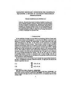
Figure 1: Coefficients κ11 (a), κ22 (b) and κ12 (c) for fixed ray gracing angles ϑ versus angle α; the curve number k corresponds to the angle ϑ = −90◦ +10◦ k; the curve at the point of reflection K = 0.02, derivatives n′z = 0.01, n′r = 0. In particular case on the free surface z = 0 and also on the horizontal bottom z = const we have

−1 2 n′z

t z κ= 0 −1

As κ12 6= 0 when n′z 6≡ 0 then horizontal planes scatter rays in inhomogeneous media. In homogeneous waveguide with n = const we obtain from (3)

t1r

− −Knt1r tr N2t tr

κ=

0 − tt1rr

To prove formula (3) let consider a narrow beam of rays, bounded by the rays with similar pulses p and p˜. Let the incident points of the rays be (r, z) e ~ and N ~, ~t, normals N and (˜ r = r + δr, z˜ = z + δz), direction vectors ~t and e respectively. From geometrical reason (Fig. 2b) we receive tr Nz ∆z, Nt tr Nr ∆z. δz ≃ − Nt δr ≃

First, we find the laws of reflection of the beam, neglecting the change of the normal vector at the site of incidence on the surface, that is, assum3

z

z N p

1

N

N

p

p

1

p

p

dz

dl

ds dl

p R

r

r

(a)

(b)

Figure 2: Scheme reflection of a narrow beam of rays from the curved surface ~ and the radius of curvature R. with normal vector N ing a flat surface. For the increment of z = z(r) − z(r) we have in this approximation d t1z δr, z1 δr = z (r) + dr t1r t˜z d z˜1 (r + δr) = z˜ (r) + z˜δr = z˜ + δr, dr t˜   r t1z t˜z − δr ≃ ∆z1 ≡ z1 (r + δr) − z˜ (r + δr) = ∆z + t1r t˜r    tr Nz t1z tz tr ≃ 1+ ∆z = − ∆z. − Nt t1r tr t1r z1 (r + δr) = z1 (r) +

4

(5)

For ∆p = p (r) − p˜ (r) we have analogously: d p1 (r + δr) = p1 (r) + p1 δr = dr  n′  p = p (r) − 2Nz Nr n2 − p2 (r) + p (r) Nz + z δr, t1r  p  2 2 p˜1 (r + δr) = p˜ (r + δr) − 2Nz Nr n (r + δr, z + δz) − p˜ (r + δr) + p˜ (r + δr) Nz , n′ d p˜δr = p˜ (r) + z δr, dr tr ∆p1 ≡ p1 (r + δr) − p˜ (r + δr) = p  p 2 2 2 2 ≃ ∆p − 2Nz Nr n − p (r) − n (r + δr, z + δz) − p˜ (r + δr) −   d d −2Nz (p (r) − p˜ (r + δr)) Nz + p1 − p˜ δr = dr dr      tz d d tz 2 2 = ∆p 1 − 2Nz + 2Nz Nr + δr+ p1 − p˜ 1 − 2Nz + 2Nz Nr tr dr dr tr n (n′r δr + n′z δz) = +2Nz Nr p 2 2 n − p (r)    t1r tr t1r 2 ′ ′ Nz = − ∆p + + − 2Nr nz + 2Nr Nz nr ∆z. (6) tr t1r tr Nt p˜ (r + δr) = p˜ (r) +

Here we have used the identity tz t1r 1 − 2Nz2 + 2Nz Nr ≡ − , tr tr   tr Nz t1z tz tr 1+ − ≡− . Nt t1r tr t1r Now take into account the effect of the curvature of the surface at the point of reflection, neglecting variations in ~t and n. Let the radius of curvature of the bottom surface is equal to R, and she curvature K = 1/R. We have dNz = d sin α = Nr dα, dNr = d cos α = −Nz dα. Differentiating (4), we obtain 5

D E D E ~ ~ ~ ~ −dt1z /2 = dNz t, N + Nz t, dN = E  D ~ + tz Nz + Nz tr dNr = = dNz ~t, N
= Nr (2tz Nz + tr Nr ) − Nz2 tr dα = −t1r dα.

Then (see Fig. 2b)

dα ≃ −Kdl = −K

δr tr = −K ∆z, Nz Nt

so when multiplied by n we get ∆p1 = 2nt1r dα ≃ −2Kn

t1r tr ∆z. Nt

(7)

After summation of (6), (7) and passing to the limit as ∆p0 → 0 we obtain (3). I wish to thank A.L. Virovlyasnky for useful discussions.

References [1] A.L. Virovlyansky. Ray theory of long-range sound propagation in the ocean (in Russian). Nizhny Novgorod: IAP RAS, 2006.

6