Feb 25, 2005 - in terms of slip length, slip velocity, pressure drop reduction (drag reduction), ... As for most problems connected with surface effects, fluid-solid inter- ... This law, and its consequences, are well verified at a macroscopic level, ...
arXiv:nlin/0502060v1 [nlin.CD] 25 Feb 2005
Mesoscopic modeling of heterogeneous boundary conditions for microchannel flows R. Benzi1 , L. Biferale1 , M. Sbragaglia1 , S. Succi2 and F. Toschi2 1 Dipartimento di Fisica, Universit`a “Tor Vergata”, and INFN, Via della Ricerca Scientifica 1, I-00133 Roma, Italy. 2 CNR, IAC, Viale del Policlinico 137, I-00161 Roma, Italy. February 6, 2008 Abstract We present a mesoscopic model of the fluid-wall interactions for flows in microchannel geometries. We define a suitable implementation of the boundary conditions for a discrete version of the Boltzmann equations describing a wall-bounded single phase fluid. We distinguish different slippage properties on the surface by introducing a slip function, defining the local degree of slip for mesoscopic molecules at the boundaries. The slip function plays the role of a renormalizing factor which incorporates, with some degree of arbitrariness, the microscopic effects on the mesoscopic description. We discuss the mesoscopic slip properties in terms of slip length, slip velocity, pressure drop reduction (drag reduction), and mass flow rate in microchannels as a function of the degree of slippage and of its spatial distribution and localization, the latter parameter mimicking the degree of roughness of the ultra-hydrophobic material in real experiments. We also discuss the increment of the slip length in the transition regime, i.e. at O(1) Knudsen numbers. Finally, we compare our results with Molecular Dynamics investigations of the dependency of the slip length on the mean channel pressure and local slip properties (Cottin-Bizonne et al. 2004) and with the experimental dependency of the pressure drop reduction on the percentage of hydrophobic material deposited on the surface – Ou et al. (2004).
1
Introduction
The physics of molecular interactions at fluid-solid interfaces is a very active research area with a significant impact on many emerging applications in material science, chemistry, micro/nanoengineering, biology and medicine, see Whitesides & Stroock (2001), Lion et al. (2003), Gad-el’Hak (1999), Ho & Tai (1998). As for most problems connected with surface effects, fluid-solid interactions become particularly important for micro- and nano-devices, whose physical behaviour is largely affected by high surface/volume ratios. Recently, due to an ever-increasing interest in microfluidics and MEMS (micro-electromechanical system)-based devices, experimental capabilities to test and analyze such systems have undergone remarkable progress. In this paper, we shall focus on flows in micro-channels, a subject which has recently become accessible to systematic experimental studies thanks to the developments of silicon technology (see Tabeling (2003), Karniadakis & Benskok (2002) and references therein). Classical hydrodynamics postulates that a fluid flowing over a solid wall sticks to the boundaries, i.e. the fluid molecules share the same velocity of the surface, Batchelor (1989); Massey (1989). This law, and its consequences, are well verified at a macroscopic level, where the characteristic scales of the flow are much larger than the molecular sizes. The situation changes drastically at a microscopic level. Many experiments (Maurer et al. (2004); Ou et al. (2004); Watanabe et al. (1999); Vinogradova & Yabukov (2003); Vinogranova (1999); Pit et al. (2000); Baudry et al. (2001); Craig et al. (2001); Zhu & Granick (2001, 2002); Cheng & Giordano (2002); 1
Tretheway & Meinhart (2002); Bonnacurso et al. (2002, 2003); Choi et al. (2003); Zhang et al. (2002)) and numerical simulations using Molecular Dynamics (Barrat & Bocquet (1999a,b); Thompson & Troian (1997); Thompson & Robbins (1990); Bocquet & Barrat (1993); Cieplak et al. (2001); Thompson & Robbins (1989); Priezjev et al. (2004)) have shown evidences that the solid-fluid interactions are strongly affected by the chemico-physical properties and by the roughness of the surface. For example, water flowing over a hydrophilic, hydrophobic or super-hydrophobic surface, may develop quite different flow profiles in micro-structures. One of the most spectacular effect is the appearance of an effective slip velocity, Vs , at the boundary, which, in turn, may imply a reduction of the kinetic energy dissipation with significant enhancement of the overall throughput (at a given pressure drop), see Watanabe et al. (1999); Vinogradova & Yabukov (2003); Pit et al. (2000); Baudry et al. (2001); Craig et al. (2001); Zhu & Granick (2001, 2002); Cheng & Giordano (2002); Tretheway & Meinhart (2002); Bonnacurso et al. (2002); Choi et al. (2003). From the slip velocity, one defines a slip length, Ls , as the distance from the wall where the linearly extrapolated velocity profile vanishes. The experimental and theoretical picture is still under active development. No clear systematic trend of the slip effect as a function of the chemico-physical components has been found to date. Slip lengths varying from hundreds of nm up to tens of µm have been reported in the literature. Moreover, controversial claims about the importance of the roughness of the surface and of the combined degree of roughness-hydrophobicity have been presented. In simple flows roughness is expected to increase the energy exchange with the boundaries, inducing a corresponding decrease in the slippage. However, both increase and decrease of the slip length as a function of the surface roughness have been claimed in the literature, Zhu & Granick (2001, 2002); Bonnacurso et al. (2002, 2003). From a purely molecular point of view, a critical parameter governing the solid-liquid interface is the contact angle (wetting angle). Clean glass is highly hydrophilic, with an angle with water close to θ = 0o (perfect wetting). Recently ultra-hydrophobic surfaces have been obtained which prove capable of sustaining a contact angle with water as high as θ = 177o a value at which water droplets are almost spherical on the surface, Chen et al. (1999); Fadeev & Carthy (1999). Some authors proposed that the increase in the slippage might be due to a rarefaction of the flow close to the wall, a depleted water region or vapor layer should exists near a hydrophobic surface in contact with water, Lum et al. (1999); Sakurai et al. (1998); Schwendel et al. (2003); Tyrrell & Attard (2001). Recent Molecular Dynamics simulations have also presented some evidences of a dewetting transition, leading to a strong increase of the slip length, below some capillarity pressure in microchannels with heterogeneous surface, Cottin-Bizonne et al. (2003, 2004). The physics looks very fragile, depending as it seems on many complicated chemical and geometrical details. From the numerical point of view, Molecular Dynamics (MD) is the standard tool to systematically investigate the problem, Frenkel & Smit (1995); Rapaport (1995); Boon & Yip (1991). In MD the solid-liquid and the liquid-liquid interactions are introduced by using Lennard-Jones type potential (with interaction energies and molecular diameters adjusted from experiments). By changing the interaction energies one may tune the surface tension and, consequently, the contact angles. MD also offers the possibility to model the boundary geometries and roughness with a high degree of fidelity. The main limitation, however, is the modest range of space and especially time-scales, which can be simulated at a reasonable computational time, typically a few nanoseconds, Rapaport (1995); Koplik & Banavar (1991). The coupling between MD and hydrodynamic modes involves a huge gap of space and time scales. Recently, an interesting attempt to reproduce MD simulations of heterogeneous microchannels with a continuum mechanical description based on Navier-Stokes equations and suitable hydrodynamic boundary conditions has been proposed, (Cottin-Bizonne et al. (2003, 2004); Priezjev et al. (2004)). Cottin-Bizonne et al. (2004) show that some of the results obtained by MD simulations of a microchannel with a grooved surface can be qualitatively reproduced using a Stokes equation for the incompressible flow, in combination with an heterogeneous boundary condition, linking the slip velocity parallel to the boundary u|| (r) to the stress in the normal direction, n ˆ:
2
u|| (r) = b(r)∂n u|| (r)
(1)
where b(r) is a position dependent normalized slip length mimicking the heterogeneity of the microscopic level. The qualitative agreement with the results of MD simulations can be obtained by properly tuning the b(r) values. In particular, they show that the dewetting transition observed in MD simulations, for some values in the Pressure-Volume diagram, is equivalent to the assumption, at the hydrodynamic level, that the boundary surface is made up of alternating strips of free-shear (high slip length b(r)) and wetting material (low slip length). In this paper, we main aim at filling the gap between the microscopic description typical of MD, and the macroscopic level of the Navier-Stokes equations by using a mesoscopic model based on the Boltzmann Equation. In particular, we will use a discrete model known as Lattice Boltzmann Equation (LBE) with heterogeneous boundary conditions. The boundary condition (1), Maxwell (1879), arises naturally in a power expansion of the Boltzmann equation in terms of the Knudsen number, Kn = λ/L, that is, the ratio between the mean free path, λ, and a typical length of the channel, L. At first order in Kn, one obtains the Navier-Stokes equation with the Maxwell boundary conditions above, Cercignani & Daneri (1963); Hadjiconstatinou (2003). Still, recent experimental results raised some doubts on the validity of this construction above some critical value of the Knudsen number, Maurer et al. (2004). There, the authors report that above Kn ∼ 0.3 ± 0.1 both helium and nitrogen exhibit a non linear dependence of the flow rate on Kn which cannot be explained by solving the Stokes equation with the first order slip boundary condition (1). For those values of Kn, the flow is in the so-called transition regime and it has been shown that the coupling between hydrodynamic equations with a second order boundary condition u|| (r) = b1 (r)∂n u|| (r) + b2 (r)∂n2 u|| (r)
(2)
is more appropriate to fit the experimental data Maurer et al. (2004). The purpose of our investigation is twofold. First, we aim at developing a model which allows a coarse-grained treatment of local effects close to the flow-surface region, without delving into the detailed molecule-molecule description typical of MD. Second, we wish to design a tool capable of describing fluid motion also beyond the linear Knudsen regime. The underlying hope behind the present hydro-kinetic approach, is that the main features of the fluid-surface interactions can be rearranged into a suitable set of renormalized LBE boundary conditions. This implies that all details of the contact angle, the solid-fluid interaction length, the local microscopic degree of roughness, can, to some extent, be included within the local definition of effective accommodation factors governing the statistical interactions between the mesoscopic molecules and the solid walls, Succi (2002); Sbragaglia & Succi (2004). In a more microscopic vein, one may also describe the interactions between solid-liquid and liquid-liquid populations using a mean-field multi-phase LBE description, see Shan & Chen (1993, 1994); Swift et al. (1995); Verberg & Ladd (2000); Verberg et al. (2004); Kwok (2003). Results based on these more sophisticated schemes will be reported in a forthcoming paper, Benzi et al. (2005). The paper is organized as follows. In section (2) we briefly remind the main ideas behind the lattice versions of the Boltzmann equations and we present a natural way to implement nonhomogeneous slip and no-slip boundary conditions in the model. In section (3) we discuss the hydrodynamic limit of the LBE previously introduced with particular emphasis on the form of the hydrodynamic boundary conditions in presence of slippage. In section (4) we present the numerical results at various Knudsen and Reynolds numbers, as well as a function of the degree of slippage and localization. Whenever directly applicable we compare the results obtained within our mesoscopic approach with (i) exact results in the limit of small Knudsen numbers obtained in the hydrodynamic formalism, Philip (1972a,b); Lauga & Stone (2003) (ii) results obtained with a microscopic approach using MD simulations, Cottin-Bizonne et al. (2004) and (iii) recent experimental results of microchannels with ultrahydrophobic surfaces, Ou et al. (2004). Conclusions and perspectives follow in section (5). Technical details are given in the appendices.
3
2
Lattice Kinetic formulation
The Boltzmann Equation describes the space-time evolution of the probability density f (r, v, t) of finding a particle at position r with velocity v at a given time t. This evolution is governed by the competition between free-particle motion and molecular collisions which promote relaxation towards a non-homogeneous equilibrium, whose distribution f eq (ρ, u), is the Maxwellian consistent with the local density, ρ(r), and coarse grained velocity, u(r). The hydrodynamic variables are obtained as low-order moments of the velocity distributions. Infact, the hydrodynamic density R R and velocity are ρ(r, t) = dvf (r, v), and u(r, t) = dvvf (r, v), respectively. The NavierStokes equations for the hydrodynamic fields are recovered in the limit of small-Knudsen numbers using the Chapman-Enskog expansion Cercignani (1991). The Boltzmann equation lives in a sixdimensional phase-space and consequently its numerical solution is extremely demanding, and typically handled by stochastic methods, primarily Direct Simulation Monte Carlo (for a review see Bird (1998)). However, in the last fifteen years, a very appealing alternative (for hydrodynamic purposes) has emerged in the form of lattice versions of the Boltzmann equations in which the velocity phase space is discretized in a minimal form, through a handful of properly chosen discrete speeds (of order ten in two dimensions and twenty in three dimensions –see appendix A for details). This leads to the Lattice Boltzmann Equations (LBE) for the probability density, fl (r, t), where r runs over the discrete lattice, and the subscript l = 0, N − 1 labels the N discrete velocities values allowed by the scheme, v ∈ {c0 , · · · cN −1 }, Succi (2001); Wolf-Gladrow (2000); Benzi et al. (1992); Chen & Doolen (1998); McNamara & Zanetti (1998). It is interesting to remark that it is sufficient to retain a limited numbers of discretized velocities at each site to recover the NavierStokes equations in the hydrodynamic limit. In two dimensions the nine-speed 2DQ9 model (N = 9) is in fact one of the most used 2d-LBE scheme, due to its enhanced stability Karlin et al. (1999). All three-dimensional simulations described in this paper are based on the the 3DQ19 scheme (N = 19) (see Fig. 10 in appendix A for a graphical description of LBE velocities in 2d and 3d). For the sake of concreteness, we shall refer to the two-dimensional nine-speed 2DQ9 model, although the proposed analysis can be extended in full generality to any other discretespeed model living on a regular lattice. We begin by considering the Lattice Boltzmann Equation in the following BGK approximation, Bhatnagar et al. (1954): � 1� (eq) fl (r + cl , t + 1) − fl (r, t) = − fl (r, t) − fl (ρ, u) + Fl (3) τ where we have assumed lattice units δx = δt = 1. In (3), τ is the relaxation time to the local equilibrium, which is proportional to the Knudsen number. The explicit expression of the speed (eq) vectors, cl , of the lattice equilibrium distribution, fl (ρ, u) and of the forcing term Fl needed to reproduce a constant pressure drop, are described in the appendix A. The hydrodynamic fields in the lattice version are expressed by: X X ρ(r) = fl (r); ρ(r)u(r) = cl fl (r). (4) l
l
Boundary conditions for Lattice Boltzmann simulations of microscopic flows have made the object of much investigation in recent years, Toschi & Succi (2005); Niu et al. (2004); Lim et al. (2002); Ansumali & Karlin (2002). In particular, we are interested in studying the evolution of the LBE in a microchannel with heterogenous boundary conditions (H-LBE) –the simplest case being a sequence of two alternating strip with different slip properties, as depicted in Fig. (1). A general way of imposing the boundary conditions in the LBE reads as follows: X Bk, (5) fk¯ (rw , t + 1) = ¯¯ l (rw )f¯ l (rw , t) ¯ l
where the matrix Bk, ¯¯ l is the discrete analogue of the boundary scattering kernel expressing the fluid-wall interactions. Here and in the following, we use the notation rw to indicate the generic spatial coordinate over the surface of the wall and the indices ¯l, k¯ label the subset of incoming and 4
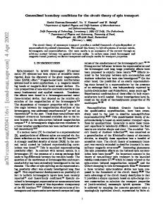
H
Lx
Lx s=s 0 s=s 1
Lz
H
Lz
s=s 0 Ly
s 0 =s 1 =s 0 s s
s=
Ly
Figure 1: Typical geometry of the microchannel configuration. We have periodic boundary conditions along the stream-wise, x ˆ, and span-wise yˆ directions. The two rigid walls at z = 0, Lz are covered by two strips of width H and L − H, where L = Lx for transversal strips (left panel) and L = Ly for longitudinal strips (right panel). The two strips have different slippage properties identified by the values s0 and s1 . The ratio ξ = H/L identifies the fraction of hydrophobic material deposited on the surface. Typical sizes used in the LBE simulations are Lx = Ly = 64 grid points and Lz = 84 grid points. This would correspond, for example, for a fluid like water at Kn = 10−3 , to a microchannel of height of the order of 100 µm.
outgoing velocities respectively. To guarantee conservation of mass and normal momentum, the following sum-rule applies: X Bk, (6) ¯¯ l (rw ) = 1. ¯ k
Upon the assumption of fluid stationarity, we can drop the dependence on t and write: X Bk, fk¯ = ¯¯ l (rw )f¯ l.
(7)
¯ l
The simplest, non trivial, application involves a slip function, s(rw ), representing the probability for a particle to slip forward, (conversely, 1 − s(rw ) will correspond to the probability for the particle to be bounced back). If we focus, for example, on the north-wall boundary condition (see Fig. (10) in appendix A), the boundary kernel upon the assumption of preserved density and zero normal component of the velocity field (6) takes the form : 1 − s(rw ) 0 s(rw ) f7 f5 f4 = f2 . 0 1 0 (8) f8 s(rw ) 0 1 − s(rw ) f6 In this language, the usual no-slip boundary conditions are recovered in the limit s(rw ) → 0 everywhere (incoming velocities are equal and opposite to the outgoing velocities), while the perfect free-shear profile is obtained with s(rw ) ≡ 1. The formalism is sufficiently flexible to allow the study of both spatial inhomogeneity of a given hydrophobic material and/or the effects of different degrees of hydrophobicity at different spatial locations. The above LBE scheme has been already successfully tested in the case of a homogeneous slippage s(rw ) = s0 , ∀rw , Sbragaglia & Succi (2004). In that case, it has been shown (see appendix B) that the LBE scheme converges to an hydrodynamic limit with the slip boundary condition u|| (rw ) = A Kn |∂n u|| (rw )| + B Kn2 |∂n2 u|| (rw )|, 5
(9)
where the parameters A, B can be tuned by changing the degree of slippage, s0 and the external forcing. In this case, the LBE reproduces the analytical prediction for the slip length, obtained by assuming the existence of a Poiseuille velocity profile and, with a suitable choice of A, B in (9), one can show that the model is also able to fit the experimental non-linear dependencies on the Knudsen number observed in Maurer et al. (2004) for nitrogen and helium.
3
Hydrodynamic limit
To begin with, we wish to analyze the hydrodynamic limit, Kn → 0, of the previous LBE models with non-homogeneous boundary conditions, as dictated by the space-dependent profile of the slip function, s(rw ), at the walls. For the sake of simplicity, we shall confine our attention to the continuum limit of zero lattice spacing and time increments, δx = δt → 0, c = δδxt → 1. Starting from the discretized equations (3) one gets for the continuum limit of the LBE: � 1� (eq) fl − fl + Fl . (10) τ In the following, we shall be interested in the case of stationary, time-independent, solutions (small-Reynolds regime). To this purpose, we may formally write the solution of (10) by using the time-independent Green’s function: ∂t fl + (cl · ∇)fl = −
fl (r) =
∞ X
i h (eq) (−1)n (τ (cl ∇))n fl (ρ, u) + τ Fl .
(11)
n=0
z Let us notice that defining τ = KnL (cs being the sound speed velocity), the above expression cs can be interpreted as a formal solution in powers of the Knudsen number. By recalling the expression of the hydrodynamic fields (4), it is readily checked that the boundary velocity can be expressed as a function of the velocity stress, ∂i uj , at the boundary itself. For sake of simplicity, we report here only the first order term (in the Knudsen and Mach numbers) of the expansion (see Appendix B): � � s(rw ) c ∂n u|| (rw ) + O(Kn2 ) (12) u|| (rw ) = Kn cs 1 − s(rw )
which is a direct generalization of the result obtained for the case of homogeneous boundary conditions (9). The main difference is that, due to the spatial dependence of the stress tensor along the wall, subtle non-linear effects may be triggered by the spatial correlation between the slip function s(rw ) and the stress at the wall. The hydrodynamic equations of motion in the stationary case read as follows: 1 (u · ∇)u = − ∇P ρ + ρ ∇ · (νρ∇u) ∇ · (ρu) = 0 � � (13) s(rw ) c 2 u|| (rw ) = Kn cs 1−s(rw ) |∂n u|| (rw )| + O(Kn ) u⊥ (rw ) = 0
where ∇P contains both the imposed mean pressure drop, F, and the fluid pressure fluctuations. In the limit of small Mach numbers ( ∆ρ ρ ≪ 1) we may take a constant density ρ = 1. Let us notice that in this limit, the incompressibility constraint ∇ · u = 0 imposes that any non-homogeneity of u|| along the wall-parallel direction must be compensated by an equal and opposite gradient of the normal velocity u⊥ . This implies that the local velocity profile cannot be of Poiseuille type everywhere (u⊥ = 0). In order to assess the effects of the slip on the global quantities, it is useful to define the mean profile, hu(z)i. Let us consider for instance the geometry depicted in Fig. (1), where the direction perpendicular to the walls is denoted by zˆ. We define an homogeneous mean profile as:
6
s0
s1
s0
Lz
Lz
Lz/2
Lz/2
0 0
Lx/4
Lx/2
3/4 Lx
s0
0
Lx
0
s1
Lx/4
Lx/2
s0
3 Lx/4
Lx
Figure 2: Results in the plane y = Ly /2 along the channel measured in the transversal strip configuration (see left panel of Fig. 1). The left panel shows the velocity profile. Notice that the pure inlet Poiseuille flow becomes an almost perfect shear free profile in the region with s1 = 1. The right panel is meant to highlight the local differences between the pure Poiseuille flow and the measured profiles, showing the result for (ux (r) − upois (r)). Notice the recirculation area, entering x deep in the channel bulk, produced by the alternating slip and no-slip boundary conditions.
1 hu(z)i = S
Z
u(r) dxdy
(14)
where h· · ·i stands for averaging over a plane parallel to the boundary surface, S. Even though the local velocity does not reproduce a Poiseuille profile, it can be shown from (13) that in the case of periodic boundary conditions between inlet and outlet flows, the mean homogeneous profile (14) cannot develop non linear stresses, namely: hu(z)i = upois (z) + uslip
(15)
with the notable fact that a slip velocity may appear at the boundary. In the above definition, (15) upois (z) stands for the Poiseuille parabolic profile with zero velocity at the boundary. A first set of qualitative results are plotted in Fig. (2), where the local velocity profiles and the difference between the observed velocities and the standard no-slip Poiseuille flow are shown. From the expression (15), one may define a macroscopic, global slip length, as the distance away from the wall at which the linearly extrapolated slip profile (15) vanishes: Ls =
uslip |∂z upois (zw )|
(16)
where |∂z upois (zw )| is the Poiseuille stress evaluated at the wall. Similarly, one may define the mass flow rate gain G as � � 6Ls Φs (17) = 1+ G≡ Φp H R being Φs = ux (r)dydz the real mass flow rate and Φp the Poiseuille mass flow rate for our configuration: � � dP L3z Ly (18) Φp = − dx 12µ with µ the dynamic viscosity of the fluid. In terms of these quantities one can define the pressure drop reduction,
7
Π=
∆Pno−slip − ∆P , ∆Pno−slip
(19)
which is defined as the gain with respect to the pressure drop corresponding to a non slip channel with the same overall throughput, Φs . The pressure drop reduction, Π, is usually interpreted as an effective drag reduction induced by the slippage, Ou et al. (2004).
4
Numerical results
Next, we present the numerical results obtained from the H-LBE model by changing the spatial distribution and intensity of the slip function at the boundaries. We shall also address dependencies of the slip flow on the Knudsen and Reynolds numbers. We begin by investigating the dependency of the macroscopic slip length, Ls , and the average mass flow rate through the channel, on the total amount of slip material deposited on the surface. The natural control parameter to investigate this issue is the average of the slip function on the boundary wall: Z 1 sav = hs(rw )i = s(rw )dS (20) S that is best interpreted as the renormalized effect of the total mass of hydrophobic material deposited on the surface, at the (unresolved) microscopic level. Second, we also present results as a function of the non-homogeneity of the hydrophobic pattern. This non-homogeneity, or roughness, can be taken as the spatial variance of the slip function: Z 1 2 2 ∆ = h(s(rw ) − sav ) i = (s(rw ) − hsi)2 dS. (21) S In order to quantify the gain or the loss in the slip flow with respect to the homogeneous situation, we shall focus our attention mainly on the simplest non-trivial inhomogeneous boundary configurations sketched in Fig. (1). This corresponds to a periodic array of two strips. In the first strip, of length H, the slip coefficient is chosen as s(rw ) = s1 . In the second strip (of length L − H), we impose s(rw ) = s0 . We will distinguish the two cases when the strips are oriented longitudinally or transversally to the mean flow. In these configurations, the total mass sav is given by: sav = ξs1 + (1 − ξ)s0 and the degree of non-homogeneity, or roughness, by: ∆2 = ξ(1 − ξ)(s1 − s0 )2 . By choosing (without loss of generality) s1 > s0 , in this configuration the quantity ξ = H/L is a natural measure of the localization of the slip effect. This geometry allows us to compare our results with some analytical, numerical and experimental results for the small Knudsen regime and also to extend the study to the transition regime. In sub-section (4.3) we shall also present results with slightly more complex boundary conditions, namely for the case of a bi-periodic pattern of alternating slip and no-slip boundary conditions.
4.1
Exact Results and Knudsen effects
As a validation test, we first check whether our model can reproduce some of the existing results concerning the slip properties of hydrodynamic systems with boundaries made up of alternating strips of zero-slip and infinite-slip lengths.
8
Philip (1972a) analyzed this situation using the Navier-Stokes equations for the case of a cylinder with boundaries made up of alternating longitudinal strips of perfect-slip and no-slip. He obtained the following exact result: ℓlong ≡ s
Ls 2 = log (1/cos(πξ/2)) Ly π
(22)
where ξ is the fraction of the plate where the slip length is infinite and where we have defined ℓlong as the normalized (to the pattern dimension) macroscopic slip length. s Notice that the r.h.s. of (22) is independent of the radius of the cylinder, and therefore Philip’s result is directly applicable to our geometry of Fig. (1), in the limit of small Knudsen numbers. More recently, Lauga & Stone (2003), analyzed the same situation with the only variant of using transversal rather than longitudinal strips. In the limit of a cylinder with infinite radius (plane wall boundaries), their result for the normalized slip length can be written as: ℓtrans ≡ s
1 Ls = log(1/cos(πξ/2)). Lx π
(23)
In our language, local infinite (zero) slip lengths can be obtained by choosing s1 = 1 (s0 = 0). A consistency check for our mesoscopic H-LBE model is to reproduce the hydrodynamic limits studied in the aforementioned papers, in the limit of small Knudsen numbers and large channel aspect-ratio, Lz /Lx . To this purpose, we performed a direct numerical simulation of the H-LBE model for a channel with square cross-section, Lx = Ly , and different heights, Lz . For small and fixed Knudsen number, by increasing the aspect ratio Lz /Lx at fixed channel length, Lx , the previous hydrodynamic limits are attained and the normalized slip lengths ℓtrans ,ℓlong are independent on Lz . In Fig. (3) s s we present the results obtained for both longitudinal and transversal strips compared with the analytical predictions (22-23) for a given channel aspect-ratio. The result (see Fig. (3)) shows that the analytical hydrodynamic results are well reproduced by our mesoscopic model. Moreover, we can go beyond the hydrodynamical limit studied by Philip (1972a,b); Lauga & Stone (2003), and investigate the effect of larger Knudsen numbers on these configurations, both in the near-hydrodynamic and in the transition regimes observed in the experiments, Maurer et al. (2004). The result (see Fig. (3)) is that an increase of the Knudsen number leads to an increase of the slip length, without preserving the ratio between ℓlong and ℓtrans (see inset of Fig. (3)). These results can be explained by observing that upon s s increasing the Knudsen number, even the ’non-conductive’ strips which had zero-slip length in the hydrodynamic regime, acquire a non-zero slip due to effects of order Kn2 in the boundary conditions, Sbragaglia & Succi (2004). As a result, the local slip length (no longer equal to zero) is incremented, thereby yielding a net gain in the overall slippage of the flow. Let us notice that at still relatively small Knudsen numbers, Kn = 0.05, a fairly substantial increase of the slip length is observed, which may reach 60 − 80% of the typical pattern dimension for a percentage of slipping surface ξ ∼ 0.8. Another interesting question concerns the dependency of the local velocity profile on the local slip properties with changing Reynolds and Knudsen numbers. We choose a transversal periodic array of strips with H = Lx /2 and s0 = 0, s1 = 1 and look at the profiles in the middle of the region with s1 = 1 and in the middle of the region with s0 = 0. The DNS results (Fig. (4)) clearly indicate a dependency on the Knudsen and Reynolds numbers only in the slip region. This is readily understood by observing that the Reynolds number is given by Re = M a/Kn, so that, by fixing the Mach number and varying the Reynolds number, we change also the Knudsen number, thus affecting the local slip properties of the flow. The most interesting result here is the inversion of concavity for the local profile nearby the wall in the slip region: a clear indication of the departure from the parabolic shape of the Poiseuille flow. Next, we check our method against some experimental results and MD simulations. For example, in Fig. (5), we show the dependency of the transversal normalized slip length, ℓtrans , as a s function of the inverse of the Knudsen number, i.e. as a function of the mean channel pressure, 9
1.2 3 Llong/Ltrans
1 0.8 Ls/L
2.5 2 1.5 1
0.6
0.5 0.3 0.4 0.5 0.6 0.7 0.8
0.4 0.2 0 0.3
0.4
0.5
0.6
0.7
0.8
ξ
Figure 3: Normalized slip length for transversal and longitudinal strips with s1 = 1, s0 = 0. We plot the normalized slip length as a function of the slip percentage ξ. The system’s dimensions are those of Fig. (1). A first set of LBE simulation is carried out at small Knudsen, Kn = 1.10−3 for transversal (�) and longitudinal strips (◦). These results are compared with the analytical estimates of Philip (1972a) (dashed line) and Lauga & Stone (2003) (continuous line). Notice the perfect agreement with the analytical results in the hydrodynamic limit. Another set of simulations is carried out with much larger Knudsen, Kn = 5.10−2 to highlight the effect of rarefaction on the system for both traversal (×) and longitudinal (+) strips. In the inset we show the ratio between the slip lengths for parallel and longitudinal strips for Kn = 1.10−3 (◦) and Kn = 5.10−2 (�). Here we notice how by increasing the Knudsen number the orientation of the strip region with respect to the mean flow becomes less important.
Lz
Lz
Lz/2
Lz/2 0 0.0
0.25
0.5
0.75
1.0
0 0.7
0.8
0.9
1.0
U/Uc
Figure 4: Local velocity profile in the middle of a slip strip (the one with s1 = 1) for transversal strips in the geometry depicted in Fig. (1). We plot the velocity in the stream-wise direction as a function of the height z for two different Reynolds numbers Re ∼ 4.5 (�), and Re ∼ 9.5 (◦). The Re numbers are estimated as the ratio between the center channel velocity of the integral profile and the sound speed velocity cs . Both velocity fields are normalized with the center channel velocity. The Knudsen numbers are Kn = 0.01, 0.005 respectively. Inset: the same but in the middle of a no-slip strip (s0 = 0)
10
0.7
Ls/Lx
0.5 0.4
4 3.5 3 2.5 2 1.5 1
0.3 0.5 0.4 10
0.3
100
Ls/Lx
G
0.6
1000
1/Kn
0.3
0.2
0.2
0.1
0.1
0.2 0.1 0
1
2 3 s0/(1-s0)
4
0 10
100
1000
0.2
1/Kn
0.3
0.4
0.5 s0
0.6
0.7
0.8
Ls , as a function of the average Figure 5: Left panel: Normalized transversal slip length, ℓtrans = L s x pressure in the system (inverse of the Knudsen number) and for different values of the localization parameter: ξ = 0.58 (�), ξ = 0.65 (◦), ξ = 0.63 (△). The values of s0 , s1 are kept fixed to s0 = 0 and s1 = 1. This behavior is qualitatively similar to what observed in MD simulations of microchannels with grooves, where the degree of slippage localization is governed by the width of the grooves, see Cottin-Bizonne et al. (2004). In the inset we show the same trends but for the mass flow rate gain G (see eq. 17). Right panel: ℓtrans as a function of the local degree of slippage s s0 for different values of slippage localization, ξ = 0.25, 0.5, 0.75 (�,◦,△ respectively). In the inset we show the dependency of the slip length, ℓtrans , on the microscopic slip properties, s0 /(1 − s0 ), s for the same values of ξ.
for different values of the localization parameter ξ. This is a direct comparison with the results in Fig. 6 of Cottin-Bizonne et al. (2004) where the evolution of the slip length as a function of the Pressure in MD simulations of a channel with grooves of different width is shown. Also in that case, the slip length increases by either decreasing the pressure (increasing Knudsen) or increasing the groove width (increasing the region with infinite slip). The two behaviors are qualitatively similar, with a less pronounced slip length for our case also due to the fact that we show the case of transversal strips while in Fig. 6 of Cottin-Bizonne et al. (2004) only the case of longitudinal grooves are presented. In the right panel of fig. (5) we plot ℓtrans at varying the level s of slippage, s0 , of one of the two strips (the other being kept fixed to s1 = 1). This is meant to investigate the sensitivity of the macroscopic observable to the microscopic details. As one can see, the change is never dramatic, at least for this configuration. In the inset of the same figure one notice a linear dependency between ℓtrans , and the local slip properties, s0 /(1 − s0 ). For s local slip properties we mean the local slip length as defined from the local boundary condition, s(rw ) |∂n u|| (rw )|. The same linear trend is observed in fig. 12 of Cottin-Bizonne et al. u|| (rw ) ∝ 1−s(r w) (2004) using a hydrodynamic model with suitable boundary conditions. In Fig. (6) we present the same kind of plot shown in the experimental investigation (see Fig. 15 of Ou et al. (2004)). Here, we plot the pressure drop reduction, Π, in the microchannel as a function of the percentage, ξ, of the free slip area on the surface (super-hydrophobic material). We note a remarkable agreement with the experimental results over a wide range of ξ, i.e. the ratio between the regions with super-hydrophobic and normal material on the wall. The geometry and Knudsen number are the same of the experiment. The only free parameters are the values of s0 and s1 assigned to the two different strips. Here, we have fixed s1 = 1 in the super-hydrophobic area, and we have varied s0 ∈ [0.4, .65] for the normal material. Notice that the LBE results exhibit the same trend of the experiments as a function of ξ and they are even in good quantitative agreement for ξ ∼ 0.6. Overall, there is a small dependency of Π on the unknown value of s0 , at least in the range considered, as already shown by the data presented in Fig. (5). Once the correct values of s1 and s0 able to reproduce the experimental results are identified, one may easily use the present LBE method to predict and extend the outcomes of other experiments with different geometries and/or distributions of the same hydrophobic material on the surface.
11
Lx
0.5
H 0.4 0.3 Π
s=s0
0.2
Lz
s 0 =s 1 =s 0 s s
0.1
s=
0.3
Ly
0.4
0.5
0.6
0.7
0.8
ξ
Figure 6: Results for the pressure drop reduction Π (19), as a function of the percentage of the free slip area on the surface. The geometry is the same investigated experimentally in Fig. 15 of Ou et al. (2004) where a micro-channel with only one surface engraved with longitudinal strips with super-hydrophobic material is studied (left panel). Here we present the results from the experiments (•), superposed with our numerical simulations (×) obtained at Kn = 5.10−4. The numerical mesh is such to mimick the same channel height of 127µm used in the experiment. The error bars in the LBE numerics represent the maximum variation obtained by fixing s1 = 1, in the shear-free area, and changing s0 ∈ [0.4, 0.65] in the normal surface.
4.2
Effects of roughness and of localization
As a next step, we address of the effect of the roughness, the total mass of the hydrophobic material, and the localization over the surface. To this purpose, we choose a transversal configuration where H = Lx /2 (fixed localization, ξ = 0.5) and s0 = sav + ∆, s1 = sav − ∆, thus yielding hsi = sav for any degree of the roughness, ∆. We then look, for a given sav , at how the slip properties of the system respond to changes in the excursion, ∆, at fixed localization ξ. The results for the normalized transversal slip length, ℓtrans , s and the mass flow rate gain, are presented in (Fig. (7)). Both the slip length and the mass flow rate increase by increasing ∆. Notice that one can easily reach slip lengths which are of the order of 10% of the channel pattern dimension by increasing the roughness at fixed total mass of slip material deposited on the surface. Similarly, the mass flow rate gain, G, is increased of the order of 20 − 30% with respect to the Poiseuille flow. In other words, the best throughput is obtained by increasing the inhomogeneity of the slippage material deposited on the surface (experimentally this means to keep the region covered by hydrophobic molecules as segregated as possible from the region covered with hydrophilic molecules). Another possible way to compute the slippage effects is to analyze the slippage at fixed total mass of hydrophobic material, varying both the localization and the roughness. To this purpose, we choose again a transversal configuration where we fix the total mass sav and we choose s1 = sav /ξ, s0 = 0, ξ = H/Lx being the degree of localization associated with a given roughness. The result (Fig. (8)) is that the slippage is greater as the the degree of localization, and –consequently– of roughness, is increased.
4.3
Mean field approach and beyond
We observe that a mean field approach is able to reproduce the qualitative trends observed so far. In the boundary condition (12) there is a coupling between the local velocity field and the stresses at the wall. Obviously, the averaged slip length depends both on s(rw ) and on the 12
1.3 G
0.1
Ls/Lx
0.08
1.2 1.1 1.0
0.06
0.0
0.1
0.2
0.3
0.4
0.04 0.02
0.0
0.1
0.2 ∆
0.3
0.4
Figure 7: Normalized transversal slip length, ℓtrans = Ls /Lx , for boundary conditions as in Fig. s (1) with s1 = sav + ∆ in a fraction ξ = H/Lx = 1/2 and s0 = sav − ∆ in the other. The Knudsen number is Kn = 0.001. We plot the normalized slip length as a function of the roughness parameter ∆ and the following values of sav are considered: sav =0.4 (�), sav = 0.5 (◦), sav = 0.6 (△). Inset: Same trends of the main body but for the mass flow rate gain G.
0.09 G
1.3
0.07
1.2
Ls/Lx
1.1 1.0
0.05
0.2
0.4
0.6
0.8
1.0
0.03
0.01 0.2
0.3
0.4
0.5
0.6 ξ
0.7
0.8
0.9
1
Figure 8: Normalized transversal slip length, ℓtrans = Ls /Lx , for boundary conditions of transvers sal strips as in Fig. (1) with s1 = sav /ξ in a fraction ξ and s0 = 0 in the other. The Knudsen number is Kn = 0.001. We plot the normalized slip length as a function of the localization parameter ξ for the following values of sav : sav = 0.25 (�), sav = 0.5 (◦), sav = 0.75 (△). Inset: Same trends of the main body but for the mass flow rate gain G.
13
stresses. In order to highlight the effect of the slip function on the mean quantities, as a first approximation, we can leave the wall stress fixed at its Poiseuille value, and work only on the properties of s(rw ), namely: s huslip i ∼ h i. (24) 1−s For the configuration analyzed so far, without loss of generality we define: δ=
s1 − s0 2
s+ =
s0 + s1 2
s and write the averaged slip properties h 1−s i as a function of δ and s+ :
h
s1 s+ − δ s0 s+ + δ s + p1 = p0 i = p0 + p1 1−s 1 − s0 1 − s1 1 − s+ + δ 1 − s+ − δ
(25)
where p1 = LHx , p0 = 1 − p1 are the percentages of the surface associated with slip and no-slip areas respectively. Making use of Taylor expansion up to second order in δ we get: h Since p1 =
H Lx
δ δ2 s+ s + (p1 − p0 ) + . i≈ 2 1−s 1 − s+ (1 − s+ ) (1 − s+ )3
(26)
= ξ and p0 + p1 = 1, we finally obtain: h
s δ(2ξ − 1)(1 − s+ ) + δ 2 s+ + . i≈ 1−s 1 − s+ (1 − s+ )3
(27)
First, in our case of a fixed localization, by setting ξ = 1/2 we have s+ = sav , δ = ∆ and we obtain: ∆2 sav s + i≈ (28) h 1−s 1 − sav (1 − sav )3 that results in a greater slippage when the roughness ∆ is increased. Second, if we choose s1 = sav ξ and s0 = 0, as for the case with fixed total mass, we obtain av av and s+ = s2ξ . This results in δ = s2ξ h
s sav sav (4ξ 2 − 2ξ)(2ξ − sav ) + 2ξs2av i≈ + 1−s (2ξ − sav ) (2ξ − sav )3
(29)
that, as a function of the localization ξ yields a qualitative agreement with our analysis, supporting the idea that the effect of slippage is greater when slip properties are localized. It should be appreciated that the mean field approach discussed above is not exhaustive. In fact, we can design an experiment with the boundary configuration sketched in Fig. (9), and investigate the total slippage as a function of the distance, d, between the strips. For this geometry, the mean field approach presented before would yield the same results irrespectively of d. On the other hand, we expect non-linear effects to be present when the strips get close enough, due to the correlation between s(rw ) and the stress at the boundary, ∂n u(rw ). Indeed, as one can see in Fig. (9), the slippage is increased when the two strips get closer to each other. This effect, even if only of the order of 10% in the mass flow rate with respect to the configuration for d ≫ 1, cannot be captured by the previous mean field argument. Let us notice that a similar sensitivity to the geometrical pattern of the slip and no-slip areas has been recently reported in the experimental investigation of Ou et al. (2004), where it is found that for the same microchannel geometries and shear-free area ratios, microridges aligned in the flow direction consistently outperform regular arrays of microposts. Similar considerations have been also presented by Vinogranova (1999).
14
0.14
Lx
0.13
s=s 0
Ls/Lx
H
0.11
1.25 0
0.1
2
4
6
8
10
0.09
d
s=s 1
G 1.35
s=s 1 Lz
1.45
0.12
s=s 0 s=s 0
1.55
0.08
H
0.07 0
Ly
2
4
6
8
10
d
Figure 9: Left: The configuration with a transversal bi-strip structure at the walls. The total boundary lengths are Lx , Ly (stream, span). The slip coefficient is chosen as s1 = 1 in two strip of length H and s0 = 0 in the others. The distance between the two strips is d. Periodic boundary conditions are always assumed in the span-wise and stream-wise direction. Right: results for the slip length and the mass flow rate gain (inset) as a function of the distance d (in lattice units) between the two free-shear (s = s1 ) strips of width H = 20 (in lattice units). All the other parameters, Lx = Ly = 64, Lz = 84, Kn = 1.10−3 are kept fixed.
5
Conclusions
We have presented a mesoscopic model of the fluid-wall interactions which proves capable of reproducing some properties of flows in microchannels. We have defined a suitable implementation of the boundary conditions in a lattice version of the Boltzmann equation describing a single-phase fluid in a microchannel with heterogeneous slippage properties on the surface. In particular, we have shown that it is sufficient to introduce a slip function, 0 ≤ s(rw ) ≤ 1, defining the local degree of slip of mesoscopic molecules at the surface, to reproduce qualitatively and, in some cases, even quantitatively, the trends observed either in MD simulations or is some experiments. The function s(rw ) plays the role of a renormalizing factor, which incorporates microscopic effects within the mesoscopic description. We have analyzed slip properties in terms of slip length, Ls , slip velocity, Vs , pressure drop gain, Π and mass flow rate Φs , as a function of the degree of slippage, and its spatial localization. The latter parameter mimicking the degree of roughness of the ultrahydrophobic material in real experiments. With a proper choice of the slip function s(rw ) in longitudinal and transversal configurations, we have reproduced previous analytical results concerning pressure-driven hydrodynamic flows with boundaries made up of alternating strips of zero-slip and infinite-slip (free-shear) lengths, Philip (1972a,b); Lauga & Stone (2003). We have also discussed the increment of the slip length in the transition regime, i.e. where the Maxwell-like slip boundary conditions (1) are supposed to be replaced by second-order ones (2). The local velocity profile has also been studied with changing Reynolds and Knudsen numbers and the local slip properties on the surface. The method introduced is able to describe slip lengths of the order of the total height of the channel (of the order of tens of µm), or fractions thereof. This is accompanied by an important increase in the mass flow rate, or equivalently, in the pressure drop gain. Whenever possible, we have compared the results based on the Heterogeneous LBE with MD simulations and with some recent experiments. In particular, we have shown that the H-LBE approach is able to reproduce the increase of the slip length as a function of the inverse of the mean pressure in the channel, as observed in recent MD simulations by Cottin-Bizonne et al. (2004). Concerning the same MD simulations,
15
Z
Y
6
2
5
15 11
2 10
0 3
12 5
17
9 3
4
1
8
7 14
7
4
8
18 X
1 6
16 13
X
Y
Figure 10: 2d and 3d lattice discretization of the velocities in the LBE schemes used in this work. The velocities entering in the north wall in the 2d scheme (left) are, f5 , f2 , f6 . The outgoing velocities are: f7 , f4 , f8 . At the south wall the roles are exchanged. we have found a similar linear dependency of the macroscopic slip lengths, Ls as a function of the microscopic slip properties at the surface. As to the experiments, we have shown that the HLBE approach is able to achieve quantitative agreement with the experimental study presented in Ou et al. (2004), concerning the slip properties as a function of the relative importance of regions with high-slip and low-slip at the surface. The natural application of our numerical tool consists in tuning the free parameters s0 and s1 in order to reproduce experimental results in controlled geometries. Then, one may use the LBE scheme with the given s0 and s1 values, to explore flows in different geometries and/or with different patterns of the same slip and no-slip materials. The method is a natural candidate to study flow properties in more complex geometries, of direct interest for applications. Transport and mixing of active or passive quantities (macromolecules, polymers etc...) can also be addressed. By definition, the present H-LBE description is limited to a phenomenological interpretation of the slip function. A natural development of this approach, is to implement a multi-phase Boltzmann description, able to attack the wall-fluid interactions and fluid-fluid interactions at a more microscopic level. This route should open the possibility to discuss the formation of a gas phase close to the wall, induced by the microscopic details of the fluid-wall physics. Results along this direction, will make the object of a forthcoming publication, Benzi et al. (2005).
6
Appendix A
The Lattice Boltzmann Equation (LBE) for a Pressure-driven channel flow is a streaming and collide equation involving the particle distribution function fl (~x, t) of finding a particle with velocity ~cl (discrete velocity phase space) in ~x at time t. The equation is written in the following form: � δ 1� x (eq) fl (~x, t) − fl (ρ, ~u) + 2 F gl (30) fl (~x + ~cl δt , t + δt ) − fl (~x, t) = − τ c with τ the relaxation time and gl the forcing term projection with the property X X gl = 0 gl~cl = 1. (31) l
l
For the case of two dimensional grid (2DQ9) depicted in Fig. (10), for example, the gl ’s can be taken with the following properties: g1 = −g3
g5 = g8 = −g6 = −g7
(32)
leaving only one unknown parameter, say g5 . Discrete space and time increments are δx , δt , with (eq) c = δδxt the intrinsic lattice velocity. The equilibrium distribution fl (ρ, ~u) is given by: � � cl · ~u)2 (~ cl · ~u) 1 (~ 1 u2 (eq) (33) fl (ρ, ~u) = wl ρ 1 + + − c2s 2 c4s 2 c2s 16
being c2s = 13 c2 the sound speed velocity. Concerning the 2DQ9 model here used for the technical details, the velocity phase space is identified by the following discrete set of velocities: ~c0 = (0, 0)c ~c1 , ~c2 , ~c3 , ~c4 = (1, 0)c, (0, 1)c, (−1, 0)c, (0, −1)c ~cα = (34) ~c5 , ~c6 , ~c7 , ~c8 = (1, 1)c, (−1, 1)c, (−1, −1)c, (1, −1)c
and the equilibrium weights are w0 = 4/9, wl = 1/9 for l = 1, ..., 4, wl = 1/36 for l = 5, ..., 8. As far as the 3d model we use in the numerical analysis (3DQ19), it is a 19 velocity model whose velocity phase space is identified by: ~c0 = (0, 0, 0)c ~c1,2 , ~c3,4 , ~c5,6 = (±1, 0, 0)c, (0, ±1, 0)c, (0, 0, ±1)c (35) ~cα = ~c7,...,10 , ~c11,...,14 , ~c15,...,18 = (±1, ±1, 0)c, (±1, 0, ±1)c, (0, ±1, ±1)c
and equilibrium weights w0 = 1/3, wl = 1/18 for l = 1, ...6, wl = 1/36, l = 8, ..., 19. Our hydrodynamic variables such as density ρ and momentum ρu are moments of the distribution function fl = fl (~x, t): X X ρ= fl ρu = ~cfl (36) l
l
and in order to derive Hydrodynamic equations from (30), we must consider the following expansions: ∞ n X ǫ fl (~x + ~cl δt , t + δt ) = Dtn fl (~x, t) (37) n! n=0 fl =
∞ X
(n)
(38)
ǫn ∂tn
(39)
ǫn fl
n=0
∂t =
∞ X
n=0
where ǫ = δt and Dt = (∂t + ~cl · ∇).order by order in ǫ and (30) imply: We can use the expansions (n) (37),(38),(39) in (30) and by equating order-by-order in ǫ self-consistent constraints on fl are obtained. Up to the first order in ǫ with ∂t = ∂t0 + ǫ∂t1 we obtain the following equations: � ∂t ρ + ∇(ρu) = 0 (40) ∂t u + (u · ∇)u = − ρ1 ∇P + ρ1 ∇ · (νρ∇u) (τ − 1 ) δ 2
with ν = 3 2 δxt and where ∇P contains both the imposed mean pressure drop, F, and the fluid pressure fluctuations.
7
Appendix B
Let us now go back to eq. (30), and derive explicitly the non-homogeneous boundary conditions used in the text (12), in the limit δx = δt → 0, with c = δδxt → 1. We specialize to the steady-state boundary condition at the north-wall (z = Lz ) for the 2d lattice (2DQ9): f7 (rw ) = (1 − s(rw ))f5 (rw ) + s(rw )f6 (rw ) f4 (rw ) = f2 (rw ) f8 (rw ) = (1 − s(rw ))f6 (rw ) + s(rw )f5 (rw ). Assuming a constant density profile ρ = 1 in the fluid, by definition we have for r = rw : u|| (rw ) = f1 (rw ) − f3 (rw ) + f5 (rw ) − f6 (rw ) + f8 (rw ) − f7 (rw ). 17
(41)
In the limit of small Mach numbers, disregarding all O(u2 ) terms in the equilibrium distribution and using the steady state, ∂t f = 0, expansion: fl (r) =
∞ X
(eq)
(−1)n (τ (cl ∇))n [fl
(ρ, u) + τ Fl ]
(42)
n=0
we finally obtain the estimate for the slip velocity u|| : u|| (rw ) = 2F τ g1 + 32 u|| (rw ) + 32 c2 τ 2 ∂x u|| (rw )+ u (r ) cτ +2s[2F τ g5 + || 6 w − cτ 6 ∂x u⊥ (rw ) − 6 ∂y u|| (rw ) +
c2 τ 2 2 6 (∂x
+ ∂y2 )u|| (rw ) +
c2 τ 2 3 ∂x ∂y u|| (rw )]
+ O(τ 3 ). (43) By noticing that the external forcing, F , is of the order of magnitude of the second-order stress, |∂y2 u|| (rw )|ν, and ν = c2s τ , the first order in Kn of (43) reads: � � s(rw ) c |∂n u|| (rw )| (44) u|| (rw ) = Kn cs 1 − s(rw ) where we have used Lz ∂y = ∂n , τ = LzcKn , ∂n u|| (rw ) = −|∂n u|| (rw )|, which is the expression s used in the text. The second-order calculation in Kn is particularly simple if we specialize to an homogeneous case (∂x (•) = 0). After some calculations, we obtain: u|| = Kn
�
c cs
�
s |∂n u|| | + Kn2 1−s
�
c cs
�2
(1 − 4g5 )|∂n2 u|| |
(45)
which is the second order, in Kn, boundary conditions, with unknown parameters s and g5 (0 ≤ g5 ≤ 1/4 ) used by Sbragaglia & Succi (2004).
References Ansumali, S. & Karlin, I. 2002 Kinetic boundary conditions in the lattice boltzmann method. Phys. Rev E 66, 026311. Barrat, J.-L. & Bocquet, L. 1999a Influence of wetting properties on hydrodynamic boundary conditions at a fluid/solid interface. Faraday Discuss. 112, 119–127. Barrat, J.-L. & Bocquet, L. 1999b Large slip effects at a nonwetting fluid solid interface. Phys. Rev. Lett. 82, 4671–4674. Batchelor, G. 1989 An Introduction to Fluid Dynamics. Cambridge University press. Baudry, J., Charlaix, E., Tonck, A. & Mazuyer, D. 2001 Experimental evidence for a large slip effects at a nonwetting fluid-surface interface. Langmuir 17, 5232. Benzi, R., Biferale, L., Sbragaglia, M., Succi, S. & Toschi, F. 2005 Mesoscopic description of the wall-liquid interaction in microchannel flows. in preparation . Benzi, R., Succi, S. & Vergassola, M. 1992 The lattice boltzmann equation: Theory and applications. Phys. Rep. 222, 145. Bhatnagar, P. L., Gross, E. & Krook, M. 1954 A model for collision process in gases. small amplitude processes in charged and neutral one-component systems. Phys. Rev. 94, 511. Bird, G. 1998 Direct Simulation Monte Carlo. Oxford. Bocquet, L. & Barrat, J.-L. 1993 Hydrodynamic boundary conditions and correlation functions of confined fluids. Phys. Rev. Lett. 70, 2726–2729. 18
Bonnacurso, E., Butt, H. & Craig, V. 2003 Surface roughness and hydrodynamic boundary slip of a newtonian fluid in a completely wetting system. Phys. Rev. Lett. 90, 1445011. Bonnacurso, E., Kappl, M. & Butt, H. 2002 Hydrodynamic force measurements: Boundary slip of water on hydrophilic surfaces and electrokinetic effects. Phys. Rev. Lett. 88, 076130. Boon, J. & Yip, S. 1991 Molecular Hydrodynamics. Dover. Cercignani, C. 1991 The Mathematical Theory on Non Uniform Gases: An Account of the kinetic Theory of Viscosity, Thermal Conduction and Diffusion in Gases. Cambridge University Press. Cercignani, C. & Daneri, A. 1963 Flow of rarefied gas between two parallel plates. J. Appl. Phys. 34, 3509. Chen, S. & Doolen, G. 1998 Lattice boltzmann methods for fluid flows. Ann. Rev. Fluid Mech. 30, 329. Chen, W., Fadeev, A., Hsieh, M., Oner, D., Youngblood, J. & McCarthy, T. 1999 Ultrahydrophobic and ultralyophobic surfaces: Some comments and examples. Langmuir 15, 3395. Cheng, J.-T. & Giordano, N. 2002 Fluid flow through nanometer-scale channels. Phys. Rev. E 65, 0312061. Choi, C., K.Johan, A.Westin & Breuer, K. 2003 Apparent slip flows in hydrophilic and hydrophobic microchannels. Phys. of Fluids 15, 2897–2902. Cieplak, M., Koplik, J. & Banavar, J. 2001 Boundary conditions at a fluid-solid interface. Phys. Rev. lett. 86, 803–806. Cottin-Bizonne, C., Barentine, C., Charlaix, E., Bocquet, L. & Barrat, J.-L. 2004 Dynamics of simple liquids at heterogeneous surfaces: Molecular dynamics simulations and hydrodynamic description. cond-mat/0404077 . Cottin-Bizonne, C., Charlaix, E., Bocquet, L. & Barrat, J.-L. 2003 Low friction flows of liquid at nanopatterned interfaces. Nature Materials 2, 237–240. Craig, V., Neto, C. & Williams, D. 2001 Shear-dependent boundary slip in an aqueous newtonian liquid. Phys. Rev. Lett. 87, 054504(1–4). Fadeev, A. & Carthy, T. M. 1999 Trialkylsilane monolayers covalently attached to silicon surfaces: Wettability studies indicating that molecular topography contributes to contact angle hysteresis. Langmuir 15, 3759. Frenkel, D. & Smit, B. 1995 Understanding Molecular Simulations. From Algorithms to Applications. Academic Press. Gad-el’Hak, M. 1999 The fluid mechanics of microdevices. Fluid Eng. 121, 5–33. Hadjiconstatinou, N. 2003 Comment on cercignani’s second-order slip coefficient. Phys. Fluids 15, 2352. Ho, C.-M. & Tai, Y.-C. 1998 Micro-electro-mechanical-systems (mems) and fluid flows. Annu. Rev. Fluid Mech. 30, 579–612. Karlin, I., Ferrante, A. & Oettinger, H. 1999 Perfect entropy functions of the lattice boltzmann method. Europhys. Lett. 47, 182. Karniadakis, G. & Benskok, A. 2002 MicroFlows. Springer Verlag. 19
Koplik, J. & Banavar, J. 1991 Continuum deductions from molecular hydrodynamics. Annu. Rev. Fluid Mech. 27, 257. Kwok, D. 2003 Discrete boltzmann equation for microfluidics. Phys. Rev. Lett. 90, 1245021. Lauga, E. & Stone, H. 2003 Effective slip in pressure-driven stokes flow. J. Fluid. Mech. 489, 55. Lim, C., Shu, C., Niu, X. & Chew, Y. 2002 Application of lattice boltzmann method to simulate microchannel flows. Phys. fluids 14, 2299–2308. Lion, N., Rohner, T., Arnaud, L. D. I., Damoc, E., Youhnovsky, N., Wu, Z.-Y., Roussel, C., Josserand, J., Jensen, H., Rossier, J., Przybylski, M. & Girault, H. 2003 Microfluidics systems in proteomics. Electrophoresis 24, 3533–3562. Lum, K., Chandler, D. & Weeks, J. 1999 Hydrophobicity at small and large length scales. J. Phys. Chem B 103, 4570. Massey, B. 1989 Mechanics of Fluids. Chapman and Hall. Maurer, J., Tabeling, P., Joseph, P. & Willaime, H. 2004 Second order slip laws in microchannels for helium and nitrogen. Phys. Fluids 15, 2613. Maxwell, J. 1879 On stress in rarefied gases arising from inequalities of temperature. Philos. Trans. R. Soc. 170, 231–256. McNamara, G. & Zanetti, G. 1998 Use of the boltzmann equations to simulate lattice-gas automata. Phys. Rev. Lett. 61, 2332. Niu, X., Shu, C. & Chew, Y. 2004 A lattice boltzmann bgk model for simulation of micro flows. Europhys. lett. 65, 600. Ou, J., Perot, B. & Rothstein, J. 2004 Laminar drag reduction in microchannels using ultrahydrophobic surfaces. Phys. Fluids 16, 4635. Philip, J. 1972a Flow satisfying mixed no-slip and no-shear conditions. Z. Angew. Math. Phys. 23, 353–370. Philip, J. 1972b Integral properties of flows satisfying mixed no-slip and no-shear conditions. Z. Angew. Math. Phys. 23, 960–968. Pit, R., Hervet, H. & Leger, L. 2000 Direct experimental evidence of slip in hexadecane: Solid interfaces. Phys. Rev. Lett. 85, 980–983. Priezjev, N. V., Darhuber, A. & Troian, S. 2004 The slip length of sheared liquid films subject to mixed boundary conditions: Comparison between continuum and molecular dynamics simulations. cond-mat/0405268 . Rapaport, D. 1995 The Art of molecular Dynamics Simulations. Cambridge University Press. Cambridge. Sakurai, M., Tamagawa, H., Ariga, K., Kunitake, T. & Inoue, Y. 1998 Molecular dynamics simulation of water between hydrophobic surfaces. implications for the long range hydrophobic force. Chem. Phys. Lett. 289, 567. Sbragaglia, M. & Succi, S. 2004 Analytical calculation of slip flow in lattice boltzmann models with kinetic boundary conditions. nlin. CG/0410089 . Schwendel, D., Hayashi, T., Dahint, R., Grunze, A. P. M., Steitz, R. & Schreiber, F. 2003 Interaction of water with self-assembled monolayers: Neutron reflectivity measurements of the water density in the inerface region. Langmuir 19, 2284. 20
Shan, X. & Chen, H. 1993 Lattice boltzmann model for simulating flows with multiple phases and components. Phys. Rev E 47, 1815–1819. Shan, X. & Chen, H. 1994 Simulation of nonideal gases and liquid-gas transitions by the lattice boltzmann equation. Phys. Rev E 47, 2941–2949. Succi, S. 2001 The lattice Boltzmann Equation. Oxford Science. Succi, S. 2002 Mesoscopic modeling of slip motion at fluid-solid interfaces with heterogeneous catalysis. Phys. Rev. Lett. 89, 064502. Swift, M., Osborn, W. & Yeomans, J. 1995 Lattice boltzmann simulations of liquid-gas and binary fluid systems. Phys. Rev. lett. 75, 830–833. Tabeling, P. 2003 Introduction a ´ la microfluidique. Belin. Thompson, P. & Robbins, M. 1989 Simulations of contact-line motion: Slip and the dynamic contact angle. Phys. Rev. Lett. 63, 766–769. Thompson, P. & Robbins, M. 1990 Shear flow near solids: Epiotaxial order and flow boundary conditions. Phys. Rev. A 41, 6830–6837. Thompson, P. & Troian, S. 1997 General boundary condition for liquid flow at solid surfaces. Nature 389, 360–362. Toschi, F. & Succi, S. 2005 Lattice boltzmann method at finite knudsen-number. Europhys. Lett. 69, 549. Tretheway, D. & Meinhart, C. 2002 Apparent fluid slip at hydrophobic microchannel walls. Phys. Fluids 14, L9–L12. Tyrrell, J. & Attard, P. 2001 Images of nanobubbles on hydrophobic surfaces and their interactions. Phys. Rev. Lett. 87, 176104. Verberg, R. & Ladd, A. 2000 Lattice-boltzmann model with sub-grid-scale boundary condition. Phys Rev. Lett. 84, 2148–2151. Verberg, R., Pooley, C., Yeomans, J. & Balazs, A. 2004 Pattern formation in binary fluids confined between rough, chemically heterogeneous surfaces. Phys. Rev. Lett. 93, 1845011. Vinogradova, O. & Yabukov, G. 2003 Dynamic effects on force measurements. lubrification and the atomic force microscopy. Langmuir 19, 1227. Vinogranova, O. 1999 Slippage of water over hydrophobic surfaces. Int. J. Miner. Process. 56, 31–60. Watanabe, K., Udagawa, Y. & Ugadawa, H. 1999 Drag reduction of newtonian fluid in a circular pipe with a highly-repellent wall. J. Fluid Mech. 381, 225–238. Whitesides, G. & Stroock, A. 2001 Flexible methods for microfluids. Phys. Today 54, 42–48. Wolf-Gladrow, D. 2000 Lattice-Gas Cellular Automata and Lattice Boltzmann Models. Springer. Zhang, X., Zhu, Y. & Granick, S. 2002 Hydrophobicity at a janus interface. Science 295, 663–666. Zhu, Y. & Granick, S. 2001 Rate-dependent slip of newtonian liquid at smooth surfaces. Phys. Rev. Lett. 87, 096105. Zhu, Y. & Granick, S. 2002 Limits of the hydrodynamic no-slip boundary condition. Phys. Rev. Lett. 88, 106102. 21