Boundary element method modelling of KEMAR for binaural rendering: Mesh production and validation KAT YOUNG1 , TONY TEW2 AND GAVIN KEARNEY3 1-3
AudioLab, Department of Electronics, University of York, Heslington, UK 1 e-mail:
[email protected] 2 e-mail:
[email protected] 3 e-mail:
[email protected] September 23rd 2016. Abstract
Head and torso simulators are used extensively within acoustic research, often in place of human subjects in time-consuming or repetitive experiments. Particularly common is the Knowles Electronics Manikin for Acoustic Research (KEMAR), which has the acoustic auditory properties of an average human head. As an alternative to physical acoustic measurements, the boundary element method (BEM) is widely used to calculate the propagation of sound using computational models of a scenario. Combining this technique with a compatible 3D surface mesh of KEMAR would allow for detailed binaural analysis of speaker distributions and decoder design - without the disadvantages associated with making physical measurements. This paper details the development and validation of a BEM-compatible mesh model of KEMAR, based on the original computer-aided design (CAD) file and valid up to 20 kHz. Use of the CAD file potentially allows a very close match to be achieved between the mesh and the physical manikin. The mesh is consistent with the original CAD description, both in terms of overall volume and of local topology, and the numerical requirements for BEM compatibility have been met. Computational limitations restrict usage of the mesh in its current state, so simulation accuracy cannot as yet be compared with acoustically measured HRTFs. Future work will address the production of meshes suitable for use in BEM with lower computational requirements, using the process validated in this work.
1
Introduction
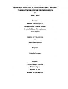
ears, whilst also varying as a function of sound source direction. However, when HTRFs are used correctly The perception of spatial sound is known to be a com- and effectively the sound field they generate at the plex phenomenon. In order to determine the location entrance to the listener’s ears is ideally identical to of a sound source, the human auditory system com- that produced by a physical sound source. bines information from a number of cues; the differMuch of binaural research centres around the acences between the signals at the ears (interaural level curate capture, analysis and synthesis of HRTFs. Unand time difference, ITD and ILD respectively) and fortunately, the experimental procedure for the capthe filtering applied by the outer ear, as well as any ture of HRTFs is time-consuming, complex and repetavailable visual cues. The ITD, ILD and the pinnae itive, requiring subjects to remain as still as possicues are all contained in a head-related transfer func- ble for long periods of time. If HRTFs are required tion (HRTF) pair. The contribution of interaural dif- within an audio reproduction system, one solution is ferences to localisation is well understood and easily to use generic HRTFs captured from a head and torso implemented within spatial audio reproduction sys- simulator (HATS) in place of the human subject. A tems, however including accurate information from particularly common HATS is the Knowles Electronthe whole HRTF, including pinnae cues, is more dif- ics Manikin for Acoustic Research (KEMAR) seen in ficult. HRTFs are unique to each individual as the Fig. 1, which has acoustical properties derived from filtering is due to the shape of the listener’s head and statistical research of the average human body, mean-
BEM modelling of KEMAR for binaural rendering
ing that KEMAR has the same acoustic properties as an average human [5]. Whilst physical acoustic measurement is perhaps the most accurate approach to capturing HRTF data, computational modelling techniques provide an appealing alternative by solving the wave equation subject to certain boundary conditions. The boundary element method (BEM) is the most common of these numerical techniques used in the calculation of HRTFs. BEM uses a surface mesh model of a scenario and defined sources and receivers to calculate the propagation of sound through the scenario. Therefore, a change in workflow to use a BEM compatible 3D surface mesh of a HATS such as KEMAR would allow for binaural analysis of speaker distributions and spatial decoder designs in a very similar way to current techniques, but without the disadvantages associated with physical measurements of human subjects. This could then be expanded to BEM calculations using mesh models of the human subjects if such meshes were available.
Young, Tew, Kearney
1.1
Boundary Element Method
To avoid measuring HRTFs, analytical and numerical methods can be used. The simplest solution for HRTF calculation is the analytical solution for scattering on a sphere, where the head is approximated as a rigid sphere without the pinnae and torso [2]. Without the pinnae the produced results are only valid for low frequencies, as the pinnae begin to have an influence above approximately 5 kHz [7]. This solution can be extended to include the torso in what is known as the ‘snowman model’ [1] but this is still missing the details in the pinnae. To account for this complex geometry, researchers developed various numerical methods, the most common of which is the boundary element method, or BEM. In BEM the boundary problem of the wave equation is converted into a surface integral, which is then discretised into a number of elements. This set of simultaneous equations can then be solved to find the pressure at a point on the surface. There are two BEM techniques used in acoustic computation: direct and indirect BEM (DBEM and IBEM respectively). DBEM is based on the Helmholtz formula, which relates the pressure in the fluid domain (in this case air) to the pressure and its normal on the boundary, and creates a nonsymmetric matrix of equations. IBEM assumes that the pressure field is caused by a monopole distribution on the boundary surface, and creates a symmetric set of equations. These equations contain a component for every element in the mesh, and there is an equation for each element. Hence, with dense meshes this equation matrix can get very large. Determining which method to use depends on the problem size. For problems over a few hundred elements the direct method is better, as it is optimised for speed. However, as it solves a full set of simultaneous equations the storage required is large. The indirect method is slower, but requires less storage [11]. In order to be used within a BEM calculation, the Figure 1: KEMAR model 45BC surface must both be closed and discretised into a mesh. This discretisation converts a smooth surface into a number of smaller planar elements, the size This paper describes the development and valida- of which determines the maximum valid frequency tion of a mesh model of KEMAR based on the orig- of the resulting calculation. It is generally acknowlinal KEMAR computer-aided-design (CAD) file. To edged that a limit of 6 elements per wavelength is acfacilitate the production of a variety of mesh models ceptable, although this can be pushed to 4 per wavesuitable for BEM calculation in the future, a workflow length. The maximum frequency is then determined is needed to ensure the resulting mesh is consistent by: with the original whilst also meeting the requirements c for BEM calculation. This process has been validated (1) fmax = edgemax × 6 using a number of analysis techniques, and opens the where c is the speed of sound in ms-1 and edgemax door for the creation of a family of meshes optimised is the length of the longest edge in m. This means for different computational situations. Interactive Audio Systems Symposium, September 23rd 2016, University of York, United Kingdom.
2
BEM modelling of KEMAR for binaural rendering
that for a mesh to be valid at 10 kHz, the maximum edge length anywhere in the mesh must be less than 5.67 mm. For 20 kHz validity, this maximum is 2.83 mm. BEM has been historically restricted to fairly low frequency calculations because of the storage requirements, but advances in computational resources are continually raising the upper frequency limit.
2
Historic Work
Weinrich was the first to attempt modelling the sound field around the head in 1984 using a number of numerical techniques [16]. The ear canal was modelled as a series of cylinders of varying radius, and the sound field calculated using transmission line theory. The sound field of a simple two-dimensional geometric model of the pinna was calculated using a finite difference time domain approach, and showed roughly the dependence of the first HRTF notch on sound source elevation. A coarse surface mesh for the head was also created, minus the pinnae, with the response calculated using BEM. The maximum validity of the mesh was only 1.7 kHz, but the results in this range compared favourably with measurements made on a physical replica of the BEM model. In the early 2000s Katz used BEM to calculate individualised HRTFs, focussing on the contribution of head and pinnae shape to the HRTF [12]. Modelling the head in a BEM environment allows for modifications such as the removal of the pinnae - crucial to investigating the contribution made to the HRTF, but not something possible with a real human subject. The work was limited by available computational resources, with 5.4 kHz being the maximum valid frequency: even after simplifying the requirements the full calculation took 50 days of CPU time. As the optical scanner used by Katz was restricted to line-of-sight only, behind the ears, the cavities of the ear, and the ear canal were all viewed as filled. This is not a problem in the case of the ear canal, as most HRTF measurements are done using a blocked ear canal. It has been shown that the ear canal does not provide any directionally dependent information [6], and ear canal-related resonance would only need to be included if the sound reproduction site were to be at the eardrum itself. The filled-in nature of the ear cavities will probably have caused errors in the final solution results, but these would likely have been above the valid frequency of the calculation. Modifications of the mesh outputted by the optical scanner were also required. The top and bottom of the mesh were closed, as the scanner could not
Young, Tew, Kearney
handle perpendicular surfaces or those which extend beyond the machine, and holes in the mesh were filled in. The mesh was then coarsened to make the computation more manageable and refined in regions where large elements existed. Katz could not locate any existing software to do this coarsening and refining, so a brute force approach was taken. Jin et al. used Fast Multipole BEM (FM-BEM) to calculate the HRTFs of a large database of subjects scanned using magnetic resonance imaging (MRI), culminating in the Sydney York Morphological and Acoustic Recordings of Ears (SYMARE) database [8]. The database contains both the meshes suitable for use within BEM at a range of frequencies and the HRTFs calculated from them. Various software applications were used in the processing workflow to perform steps similar to those described by Katz [12]. The SYMARE database is available at a number of frequency resolutions: 6 kHz, 8 kHz, 10 kHz, 12 kHz, and 16 kHz, whilst the head-only mesh is available at 15 kHz, 16 kHz and 20 kHz. An average mesh has approximately 130,000 elements. The Amira software [3] was used to extract the surface meshes from the scan data. Geomagic Studio (now discontinued, replaced by Geomagic Wrap [4]) was then used to clean the mesh and fill in holes (ear canal, nose etc). Geomagic Studio and the open source software MeshLab [13] were used to complete the various alignments and merges required across mesh resolutions. The open source software ACVD [15] was then used to improve uniformity of the surface elements across the mesh, and Geomagic Studio used again to reduce the number of elements by applying a small amount of smoothing. In a large body of work culminating in [10], Kahana and Nelson used a laser-scanned model of KEMAR in BEM calculations to look at contributions made by the pinnae to the HRTF (known as pinna-related transfer functions: PRTFs) by using both KEMAR and a baffled pinnae, in similar work to Katz. Their results were also limited in frequency due to the available computational resources, with the calculations valid below 10 kHz. The scanned surface was decimated using an algorithm by Johnson and Hebert [9] to create a more homogenous distribution of nodes and elements, creating a mesh with 23,000 elements valid up to 10 kHz (using the rule-of-thumb of 6 elements per wavelength). Their work showed the feasibility of BEM usage up to higher frequencies, but full mesh calculation was still limited by computation requirements. The baffled pinnae mesh was valid up to 20 kHz due to the physically smaller size of the mesh. Previous work using KEMAR within BEM has
Interactive Audio Systems Symposium, September 23rd 2016, University of York, United Kingdom.
3
BEM modelling of KEMAR for binaural rendering
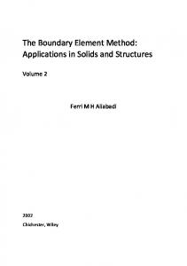
and 3b), most likely due to larger flatter areas of the torso defined using fewer mesh elements. As the maximum valid frequency is dependent on the largest edge length present in the mesh, a remeshing procedure was required to create a mesh that is valid up to 20 kHz by breaking up these large flat regions and reducing the edge lengths. 2
×105
1.5
Frequency
relied on a scanned version of some form. This has been shown to have certain limitations. Often scanners are restricted to line-of-sight, meaning occluded areas cannot be captured. This leads to regions such as behind the ear and resonant cavities within the ear being seen as filled [12], an obvious difference when compared to an actual pinna. Important morphological details can also be lost if the scan is not of a high enough resolution [10], as well as requiring post processing to combine scans from multiple directions. In the present work, however, the original CAD file of KEMAR used to produce the physical dummy is used rather than a scan, meaning complete accuracy can in principle be obtained.
Young, Tew, Kearney
1
0.5
Methodology
Following the work of Jin et al. [8], a number of software applications were used to create a mesh suitable for BEM usage from the initial CAD file. The CAD information describes the entirety of KEMAR, including torso and base. Perfect consistency with the physical KEMAR was therefore theoretically possible, and the model should not suffer from the disadvantages associated with some scanning techniques. Once created by the designer, the 3D shape in the CAD file is described using a series of large faces, defined by cartesian coordinate points and curved splines known as boundaries. These large curved faces can be seen in Fig. 2. This type of definition is unsuitable for BEM calculation, so conversion was required to create a discretised planar polygonal mesh.
0 0
5
10 15 20 Edge Length (mm)
25
30
(a) Prior to remeshing: full histogram 700 600 Frequency
3
500 400 300 200 100 0 5
10
15 20 Edge Length (mm)
25
(b) Prior to remeshing: tail of histogram 8
×104
Frequency
6 4 2 0 0
1
2 3 Edge Length (mm)
4
5
(c) After remeshing: full histogram Figure 3: Distribution of edge lengths in mesh before and after remeshing Figure 2: Head portion of the KEMAR CAD file
Geomagic Wrap [4] was used to convert the CAD file to a polygonal mesh, defined by information contained within the STEP CAD file format. The resulting mesh had 200,014 vertices and 400,001 faces, but with an irregular and undesirable distribution of shape and size. The maximum edge length in this mesh was 28.3 mm (as can be seen in Figures 3a
The ‘remesh’ feature of Geomagic Wrap was used to redefine the surface mesh with a target edge length of 2 mm. This process resulted in a mesh with a much improved distribution of edge lengths (as seen in Fig. 3c); whilst not all are under the target length of 2 mm, the largest is only 4.04 mm, giving a maximum valid frequency of 14 kHz when assuming 6 edges per wavelength. This is better than the original mesh, but still not ideal. The shape of some faces
Interactive Audio Systems Symposium, September 23rd 2016, University of York, United Kingdom.
4
BEM modelling of KEMAR for binaural rendering
Young, Tew, Kearney
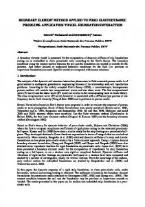
was also undesirable, in that they were too long and thin. Equilateral triangles are much preferred over long thin triangles. To create more nearly equilateral triangles across the mesh, the open source software ACVD [15] was used. This improved the distribution of edge lengths, as seen in Fig. 4. The maximum edge length was reduced to 2.49 mm (valid to 22.7 kHz when assuming 6 edges per wavelength) but at the expense of many more vertices and faces. Figure 5: Pinna portion of the final mesh 10
×104
Frequency
8
4
Validation
A number of validation steps were required during the process of mesh production to inform decisions. 4 As detailed in the previous section, maximum edge 2 length and volume were the primary criteria for validity at each stage of the process. 0 0 0.5 1 1.5 2 2.5 In addition to the maximum edge length criteEdge Length (mm) rion, BEM solvers often have a minimum and maximum internal angle requirement to help avoid the Figure 4: Distribution of edge lengths in final mesh inclusion of long thin triangles. In this and related future work, the PACSYS PAFEC-FE software [14] is the intended BEM solver, which enforces angles to The remeshing process introduced a large number be between 15°and 150°. All angles in the final mesh of unreferenced vertices: more specifically, the proce- were between these limits (as seen in Fig. 6), with the dure did not remove the vertices associated with the minimum at 16.0°and maximum at 146.7°. previous arrangement of triangles, resulting in more ×105 vertices than were used. This did not affect the struc2 ture of the mesh, but would require a BEM solver to 1.5 do more calculations than was strictly needed. The open source software MeshLab [13] was used between 1 Geomagic Wrap and ACVD to remove these unreferenced vertices. 0.5 Frequency
6
The final mesh had 360,017 vertices and 720,015 faces, a portion of which including the pinnae appears in Fig. 5. It can been seen that the mesh contains consistently small equilateral triangles.
Figure 6: Distribution of angles in the final mesh
The volume of the mesh at each stage of processing was also calculated to ensure no large discrepancies were introduced, as a change in volume from the original mesh invalidates any BEM calculations. These volume calculations, and their difference from the original CAD file, can be seen in Table 1. There is a very small loss of volume at each stage that can be attributed to the slight rounding of sharp corners during the remeshing and redistribution processes, however no particular stage introduced a large variation in volume, suggesting that all software applications and processes used were valid. This is investigated further in the next section.
The local topology of the mesh was also of importance to ensure no regions were distorted by the process, so the distances between the faces in the original CAD data and the processed mesh were calculated. These values show that the local topology is consistent with the original, with all values less than 0.64 mm and the majority less than 0.1 mm; some faces had zero distance between them. This distribution can be seen in Fig. 7. The larger distances lie in regions such as the edge of the base and within the eyes, where the radius of curvature can be relatively small and the shape has been rounded during
0 0
20
40
60 80 100 Angle (degrees)
Interactive Audio Systems Symposium, September 23rd 2016, University of York, United Kingdom.
120
140
160
5
BEM modelling of KEMAR for binaural rendering
Mesh Original CAD file Initial mesh Remeshed at target edge length Redistributed mesh
Young, Tew, Kearney
Volume (mm3 ) 28492978 28489372 28488486 28486546
Difference from original 0% -0.0127% -0.0158% -0.0226%
Table 1: Volume calculations for each stage of processing - mm3 is required for the differences to be visible.
Frequency
Frequency
×105 the remeshing or redistribution process. These re5 gions are not of critical importance to the BEM cal4 culation however; the values in the region around the pinnae are of higher importance. Whilst not zero, the 3 values here are small enough to be considered valid, 2 although further testing is required to confirm this 1 for different applications. Fig. 8 shows the distances between the faces as a function of colour, with black 0 0 0.1 0.2 0.3 0.4 0.5 0.6 0.7 at zero and white at the maximum value of 0.63mm. Distance between meshes (mm) Whilst the pinna lights up a small amount, there is (a) Full histogram not as much white as in other regions of the mesh. 2000 Unfortunately, whilst the mesh is numerically valid for BEM and consistent with the original CAD 1500 file, the size of the mesh renders it unusable by current solvers. A mesh consisting of 720,015 faces 1000 would require 7725GB of RAM to store the necessary equations to then solve using the PAFEC-FE 500 software. This means that HRTFs of KEMAR cannot be calculated using this version of the mesh: a 0 0.1 0.2 0.3 0.4 0.5 0.6 0.7 physically smaller mesh or one with a lower frequency Distance between meshes (mm) limit would be required. Additionally, even if the (b) Tail of histogram mesh could be used for BEM calculation of HRTFs, this mesh includes the ear canals, and there are no Figure 7: Distribution of distances between the two databases of acoustically measured KEMAR HRTFs meshes which include the ear canal to compare against.
Interactive Audio Systems Symposium, September 23rd 2016, University of York, United Kingdom.
6
BEM modelling of KEMAR for binaural rendering
Young, Tew, Kearney
Figure 8: Distances in mm between the two meshes, plotted on the final mesh as a colourmap
5
Conclusion
ferent frequency ranges. Physical mesh size could also be adjusted: a mesh consisting of only head The original KEMAR CAD file was converted using and shoulders would be sufficient for the majority a number of processing stages to a mesh which meets of HRTF calculations, whereas the entire torso of the topological constraints for BEM compatibility. KEMAR is present here. A mesh without ear canals The original 3D surface data has been discretised, would also be of more use than the current mesh, alremeshed and redistributed to meet the edge length lowing comparison between typical acoustically mearequirement for a 20 kHz maximum valid frequency sured HRTFs and those calculated using BEM. and the angle limitations imposed by the BEM solver. The volume and topology of the meshes prior to and after processing have been compared to ensure con- 6 Acknowledgements sistency between the original and the final mesh, and whilst there are small differences these are likely to This work is supported by Meridian Audio Ltd and be within the margin of error introduced when com- MQA Ltd. Thanks also to Mr Laurence Hobden, Mr paring a calculated result with a physically measured Patrick Macey and Mr John King from PACSYS, and result. The workflow created in this paper is applica- to G.R.A.S for supplying the CAD file of KEMAR. ble more generally to the processing of meshes edited from an original, with consistency and validity assumed. References
5.1
Further Work
Due to computational limitations the final mesh is not usable in BEM calculations in its current state. The primary aim of this work was to determine the workflow required to accurately convert the CAD information into a BEM-friendly mesh; further work is needed to address the problem of computation and usage. This could include a reduction in maximum valid frequency, by permitting longer edges and therefore larger faces, or by using different meshes for dif-
[1] V Ralph Algazi, Richard O Duda, Ramani Duraiswami, Nail A Gumerov, and Zhihui Tang. Approximating the head-related transfer function using simple geometric models of the head and torso. The Journal of the Acoustical Society of America, 112(5):2053–2064, 2002. [2] Richard O. Duda and William L Martens. Range dependence of the response of a spherical head model. The Journal of the Acoustical Society of America, 104(5):3048, nov 1998.
Interactive Audio Systems Symposium, September 23rd 2016, University of York, United Kingdom.
7
BEM modelling of KEMAR for binaural rendering
[3] FEI. Amira 3D Software for Life Sciences, 2016. [4] Geomagic. Geomagic Wrap 3D Imaging software, 2016.
Young, Tew, Kearney
human heads and baffled pinnae using accurate geometric models. Journal of Sound and Vibration, 300:552–579, 2007.
[11] Brian F. G. Katz. Boundary element method calculation of individual head-related transfer function. I. Rigid model calculation. The Journal of D Hammershøi and H Møller. Sound transmisthe Acoustical Society of America, 110(5):2440, sion to and within the human ear canal. The 2001. Journal of the Acoustical Society of America, 100(1):408–27, 1996. [12] Brian F. G. Katz. Boundary element method calDavid Howard and Jamie Angus. Pinnae and culation of individual head-related transfer funchead movement effects. In Acoustics and Psytion. II. Impedance effects and comparisons to chacoustics, chapter 2.6.3, page 103. Focal Press, real measurements. The Journal of the Acousti2 edition, 2001. cal Society of America, 110(5 Pt 1):2449–55, nov 2001. Craig Jin, Pierre Guillon, Nicolas Epain, Reza Zolfaghari, Andr´e Van Schaik, Anthony I Tew, [13] MeshLab. MeshLab, 2016. Carl T Hetherington, and Jonathan B Thorpe. Creating the Sydney York Morphological and [14] PACSYS Ltd. PAFEC-FE, 2016. Acoustic Recordings of Ears Database. IEEE [15] S. Valette, J.-M. Chassery, and R. Prost. Transactions on Multimedia, 16(1):37–46, 2014. Generic Remeshing of 3D Triangular Meshes with Metric-Dependent Discrete Voronoi DiaAndrew E Johnson and Martial Hebert. Control grams. IEEE Transactions on Visualization and of polygonal mesh resolution for 3-d computer Computer Graphics, 14(2):369–381, 2008. vision. Graphical Models and Image Processing, 60(4):261–285, 1998. [16] Søren Gert Weinrich. Sound field calculations Yuvi Kahana and Philip A Nelson. Boundary around the human head. Acoustics Laboratory, element simulations of the transfer function of Technical University of Denmark, 1984.
[5] G.R.A.S. Head & Torso simulators, 2016. [6]
[7]
[8]
[9]
[10]
Interactive Audio Systems Symposium, September 23rd 2016, University of York, United Kingdom.
8