Boundary Value Testing Using Integrated Circuit Fault Detection Rule Ruilian Zhao1 Zheng Li Department of Computer Science CREST, Department of Computer Science Beijing University of Chemical Technology King’s College London Beijing 100029, China Strand, London WC2R 2LS, United Kingdom.
[email protected] [email protected]
Abstract Boundary value testing is a widely used functional testing approach. This paper presents a new boundary value selection approach by applying fault detection rules for integrated circuits. Empirical studies based on Redundant Strapped-Down Inertial Measurement Unit (RSDIMU) of the 34 program versions and 426 mutants compare the new approach to the current boundary value testing methods. The results show that the approach proposed in this paper is remarkably effective in conquering test blindness, reducing test cost and improving fault coverage. Keywords: Boundary Value Testing, Test case generation, fault detection
1
Introduction
An investigation showed that U.S. users suffered annual economic losses total more than $59 billion. More important from the viewpoint of developers is that more than onethird of these losses could have been removed with the help of software testing [26]. Therefore, software testing is an essential technique for ensuring software quality and reliability. One of most difficult and expensive problems in software testing is the effective generation of test cases. To test a program, it is necessary to select test cases from the domain of input variables. Testing all possible inputs would provide the most complete behavior of a program, but the input domain is usually too large to be completely exercised. Instead, an usual way is to select a relatively small subset, which is a representative of the input domain in some sense [21]. Therefore, a key problem in software testing is how to develop test cases from the input domain to detect as many faults as possible with a minimum cost. 1 On
sabbatical leave to King’s College London.
There are a large number of test cases generation strategies, such as random testing [4, 8], equivalence partitioning [1, 23], boundary value testing [9, 16, 22], path testing [15, 8], and domain testing [12, 29]. Testers have frequently observed that domain boundaries are particularly fault-prone and should therefore be carefully checked. Howden and Foster [11, 7] gave careful analyses of the error sensitivity of boundary values testing. Some studies on retrospective fault data showed that boundary value testing outperforms all the other methods, by comparing statement coverage, branch coverage, random testing, boundary value testing and several other testing approaches to find these faults [1, 20]. Standards such as IEC61508 permit the use of boundary values to reduce the number of test cases. As the name suggests, boundary value testing focuses on software testing efforts at the extreme ends of the input domain. There are some existing boundary value testing methods, including boundary value analysis (testing), robustness testing, worst case testing and robustness worst case testing. However, some of these methods are hardly used in the practical software testing, because a large amount of test cases are required, thus the test generation is hard to manipulate. As we know, there are many mature testing technologies in hardware systems. It gives us an inspiration of using fullgrown hardware approaches in testing for software. In this paper, we present a novel boundary value testing approach based on the principle of fault diagnosis in integrated circuits. Moreover, a corresponding automatic test cases generation tool is developed. According to a real-world application Redundant Strapped-Down Inertial Measurement Unit (RSDIMU) specification, we design three boundary test suites. Two of them are produced by using current boundary value testing methods, the third is developed by the new boundary testing approach proposed in this paper. 34 RSDIMU program versions and 426 mutants conducted by Chinese University of Hong Kong (CUHK) are checked
by these test suites. All 426 mutants are killed and 8 new software faults are found. The experiment results show that the new boundary value testing approach, compared with existing boundary testing method, is of less test cases, and of high capability in detecting faults. The efficiency of software testing can be thus largely improved. The primary contributions of the paper are as follows: 1. A novel boundary value testing approach by applying fault detection rules for integrated circuits to boundary value selection is proposed. 2. Empirical study based on 34 RSDIMU program versions and 426 mutants provides the evidence that the new approach proposed in this paper produces much smaller test suites while keeping strong fault detection ability. The remainder of this paper is organized as follows. Section 2 briefly introduces existing boundary value testing methods. Section 3 describes main principle of the test cases selection by the new boundary value testing approach. Section 4 presents an experimental study to show how to use the method in practice. Section 5 discusses the experimental results. Section 6 reviews related work in this area. Finally, conclusion is provided in Section 7.
2
Boundary value testing methods
Boundary value testing is one of most effective functional testing strategies in common use. The idea and motivation behind boundary value testing is that errors are most likely to occur at those points when input values change from valid to invalid. Existing boundary value testing methods include boundary value testing, robustness testing, worst case testing and robustness worst case testing [9, 10, 14, 30]. 1. Boundary Value Testing (BVT) The basic idea of applying boundary value testing on the program under test is to maintain all but one of the input variables at their normal (or average) values and the remaining variables are set its extreme values in turn. The values used to test the extremities are: the minimum value, a bit more than the minimum value, normal value, a bit less than the maximum value, and the maximum value, referring to min, min+, nom, max− and max, respectively. There is one instance that all variables take their nominal value. The test cases selection in a program with two input variables is shownin Figure 1(a), where x1 (a ≤ x1 ≤ b) and x2 (c ≤ x2 ≤ d) are input variables of the program. As there are four extreme values, 4n+1 test cases should be developed for a program with n input variables.
2. Robustness Testing (RT) Robustness testing is an extension of boundary value testing, and it pays more attention on exception behaviors of the system under test.In addition to the aforementioned five testing values min, min+, nom, max− and max, robustness testing uses two more values for each variable i.e., min− and max+, which are designed to capture the values just outside of boundaries of the input domain. The test cases selection in a program with two variables is shown in Figure 1(b). Each variable has to take on its six different extreme values, respectively, and the other variables hold their nominal value. As a result, 6n+1 test cases should be designed for a program with n input variables. 3. Worst Case Testing (WCT) Worst case testing performs the Cartesian product in terms of the original five element sets: min, min+, nom, max− and max. The principle of test point selection in a program with two variables is shown in Figure 1(c). We can see from Figure 1(c) that worst case testing is more comprehensive. As each variable has to take five values for each permutation, 5n test cases are generated for a program with n input variables. Obviously, the test suite produced using boundary value testing is a proper subset of that using worst case testing. 4. Robustness Worst Case Testing (RWCT) Robustness worst case testing, as its name implication, draws it attributes from robustness testing and worst case testing. The method makes the Cartesian product in terms of the seven element sets: min−, min, min+, nom, max−, max and max+. Figure 1(d) gives the test cases selection in a program with two variables. For a program with n input variables, 7n test cases need to be generated as each variable require to hold seven values. Clearly, the test suite of robustness testing is a proper subset of that of robustness worst case testing. Boundary value testing and robustness testing are based on single-fault assumption in software reliability theory. The assumption relies on the statistic that failures are only rarely the product of two or more simultaneous faults. If we disregard the single fault assumption, this is to say, we believe software failures are caused by two or more than two simultaneous faults. It is called multi-faults assumption in reliability theory. Consequently, (robustness) worst case testing is based on the multi-faults assumption. The outcomes of the program under test are checked when more than one variables are taken its extreme values. As expected, it results in a larger set of tests and requires more
x2
x2
d
d
c
c
a
b
x1
a
(a) Boundary value testing
x1
b
x1
(b) Robustness testing
x2
x2
d
d
c
c
a
b
b
x1
(c) Worst case testing
a
(d) Robustness worst case testing
Figure 1. Principles of test point selection in a program with 2 input variables efforts to produce. Therefore, (robustness) worst case testing is generally used in the situations that high reliability is required and the consumption of time and efforts may not be taken into account. For many software, this can be too expensive to be put in practice. However, some researches showed that 20% ∼ 40% software faults are caused by only a system parameter, and another 20% ∼ 40% software faults are involved in the interactions of two or more than two parameters [17]. As a result, some common software faults will be not detected while using test cases designed based on single-fault assumption. In this paper, a novel approach of boundary test cases generation based on the multi-faults assumption is proposed.
3
A novel boundary test generation approach
This section presents how to generate efficient boundary test cases based on the principle of fault detecting in digital system. Stuck-at fault diagnosis has been one of the well-known techniques in integrated circuit testing. A Stuck-at fault is a particular fault model which is applied to gate level circuits. These faults are called stuck-at-0 or stuck-at-1 fault. To check whether a gate circuit return the right outputs, a test vector need to be developed to indicate that the circuit
is faulty or not. Moreover, some research results illustrate that a series of tests for stuck-at faults can often find a large number of other faults [25]. This paper proposed a novel approach to developing software boundary test cases base on the test vector generation for stuck-at faults in integrated circuits. Let F be the function of a software under test, F : (x1 , x2 , · · · , xn → y1 , y2 , · · · , ym ) where xi (i = 1, 2, · · · , n) is an input variable and yj (j = 1, 2, · · · , m) is an output variable of the function F . The domain Dxi is a set of all values that input variable xi can hold. Let D be the domain of a function F , D is a Cartesian product D = Dx1 × Dx2 × · · · × Dxn = {(x1 , x2 , · · · , xn )|∀x1 ∈ Dx1 , x2 ∈ Dx2 , · · · , xn ∈ Dxn }. A single point x(x ∈ D) is referred to as a function input. Let I = (x1 , x2 , · · · , xn ) be the vector of input variables, and E denotes a space of n-dimension vectors, namely input space. Thus, the domain D of a function can be thought of a subset of input space E. Assume that the distance between two points is defined as the length of the line segment between them. The domain D is said to be bounded if there exists a positive number δ such that every point x = (x1 , x2 , · · · , xn ) ∈ D satisfies |xi | ≤ δ for all i = 1, 2, · · · , n. A point q (q ∈ D) is called a boundary point if, for every neighborhood N (q)
of q, there exists q ′ , q ′′ ̸= q such that q ′ ∈ N (q) ∩ D and q ′′ ̸∈ N (q) ∩ D. Here a neighborhood N (q) of points q is a set consisting of all points x′ whose distance with q is less than a small positive numeral r. Boundary of domain D is composed of all the boundary points of domain D. Definition 1. The projection of domain D on xi axis The projection of domain D on xi axis, represented by D|xi , is a subset of the one dimension space Dxi , where D|xi = {xi ∈ Dxi |∃(x01 , · · · , x0i−1 , xi , x0i+1 · · · , x0n ) ∈ D} It can be drawn that the minimum value and the maximum value of D|xi are two boundary points. They are denoted by ximin and ximax respectively, and ximin ≤ xi ≤ ximax . If replacing the value of ximin and ximax with logical value 0 and 1, respectively, the domain Dxi can be represented as Di′ = {x′i }, where 0 ≤ x′i ≤ 1, (i = 1, 2, · · · , n). As a result, the domain D is presented as follows: D = D1′ × D2′ × · · · Dn′ = {(x′1 , x′2 , · · · , x′n )|0 ≤ x′i ≤ 1} Considering from the logical input value, functions F can be thought of an logical circuit with n inputs, as shown in Figure 2. D1 D′ D2 D′
. . . Dn D′
Figure 2. Logical circuit with n inputs. According to the principle of fault detection in the logical circuits, a set of test vectors (0, 1, · · · , 1), (1, 0, 1, · · · , 1), · · · , (1, 1, · · · , 0, 1) and (1, 1, · · · , 1, 0) should be developed to check input faults and stuck-at-1 faults for an AND gate with n inputs. In addition, another test vector (1, 1, · · · , 1) is required to detect stuckat-0 faults. For a OR gate with n inputs, a set of test vectors (1, 0, · · · , 0), (0, 1, 0, · · · , 0), · · · , (0, 0, · · · , 1, 0) and (0, 0, · · · , 0, 1) is demanded to discover stuck-at-0 faults, and another test vector (0, 0, · · · , 0) is needed to reveal stuck-at-1 faults. In total, there are 2n+2 test vectors needed [28]. To generate boundary test cases for a software with n input variables, we need to consider boundary points of input domain D, inside points of the boundary, and outside points of the boundary. Therefore, we focus on the boundary and robust value of each input variable of the software under test, namely consider each variable xi takes its ximin , ximax , and beyond ximin and ximax by adding
or subtracting a small offset ε(ε > 0), respectively. As a result, test cases of n-dimension variables are designed as follows: (x1min , x2min , · · · , xnmin ) (x1max , x2max , · · · , xnmax ) (x1min − ε, x2min , · · · , xnmin ) (x1min , x2min −ε, · · · , xnmin ) ··· (x1min , x2min , · · · , xnmin −ε) (x1max +ε, x2min , · · · , xnmin ) (x1min , x2max +ε, · · · , xnmin ) ··· (x1min , x2min , · · · , xnmax +ε) (x1max +ε, x2max , · · · , xnmax ) (x1max , x2max +ε, · · · , xnmax ) ··· (x1max , x2max , · · · , xnmax +ε) (x1min −ε, x2max , · · · , xnmax ) (x1max , x2minx −ε, · · · , xnmax ) ··· (x1max , x2max , · · · , xnmin −ε) There are 4n+2 test cases required in total. Obviously, these test cases fall on the boundary of domain D or near it from outside. Some additional test cases within domain D, similar to existing boundary value testing, need to be considered. But, different from existing methods where normal or average values are taken into account, we consider the value within domain D and near the boundary. All test cases locate outside of domain D except two settling on its boundary. Thus, test cases within domain D can be developed by adding or subtracting a small offset on the two valid boundary test cases, which are designed as follows: (x1min +ε, x2min +ε, · · · , xnmin +ε) (x1max −ε, x2mmx −ε, · · · , xnmax −ε) As a result, 4n+4 test cases are required by the new boundary test generation approach. For example, as shown in Figure 3, for a program with two inputs, 12 test cases need to be developed. It can be seen that points 1 and 2 fall on the boundary of domain D, points 3–10 are without the domain D, and points 11 and 12 are within the domain D. These test points and corresponding extreme values are given below the diagram.
x2
4 6
d
2
9
This section shows how to use the new boundary testing approach to develop test cases according to a real application project RSDIMU.
7
12
11
c
1 3 5 7 9 11
3
4.1
1
Subjects
5
4
10
a
b
(x1min , x2min ) (x1min − ε, x2min ) (x1max +ε, x2min ) (x1max +ε, x2max ) (x1min −ε, x2max ) (x1min +ε, x2min +ε)
2 4 6 8 10 12
x1
(x1max , x2max ) (x1min , x2min −ε) (x1min , x2max +ε) (x1max , x2max +ε) (x1max , x2min −ε) (x1max −ε, x2max −ε)
Figure 3. Boundary test points selection for the new approach.
The number of test cases required by four existing and the new boundary testing approach, with different input variables, are listed in Table 1. It is obvious that the number of test cases of the new approach is much less than that of (robustness) worst case testing. For example, for the programs with 10 input variables, WCT and RWCT require separately 9765625 and 282475249 test cases, but the new approach only needs 44 test cases. In addition, the new test cases set is a proper subset of robustness worst case testing. According to the test cases selection principle, we developed a test generation tool to implement automatic generation of 4n+4 boundary test cases.
Table 1. Number of test cases with different input variables.
BVT
RT
WCT
RWCT
5 9 13 17 21 25 29 33 37 41
7 13 19 25 31 37 43 49 55 61
5 25 125 625 3125 15625 78125 390625 1953125 9765625
7 49 343 2401 16807 117649 823543 5764801 40353607 282475249
The Redundant Strapped-Down Inertial Measurement Unit project (RSDIMU) was first developed for a NASAsponsored 4-university multi-version software experiment [6]. It is part of the navigation system in a spacecraft. In this application, the vehicle acceleration is estimated using the eight accelerometers mounted on the four triangular faces of a semi-octahedron in the vehicle. According to the RSDIMU specification, 20 program versions were developed, which were systematically tested by 1200 test cases designed by aviation industry experts and scholars. In 2002, the Chinese University of Hong Kong involved more than one hundred students on the same specification and 34 program versions were developed within 12 weeks. 1200 test cases were applied to acceptance testing after RSDIMU programs developed. All the 34 program versions passed acceptance test after faults detecting, removing and retesting. 21 program versions were selected for creating mutants. The other 13 versions were disqualified as their developers did not follow the development and coding standards which were necessary for generating meaningful mutants from their projects. Software faults, which were detected during the stage of unit testing, integration testing and acceptance testing, were injected into the final program versions, and 426 mutants were created, each contains one programming fault. Each program version’s size in terms of the Source Lines of Code (SLoc), the number of functions, and number of mutants developed from each program version are shown in Table 2. The details of the project and development procedures are discussed in [19, 2].
4.2
Number of test cases #Inputs 1 2 3 4 5 6 7 8 9 10
Experimental Study
8
New BVT
8 12 16 20 24 28 32 36 40 44
Boundary test cases generation
There are two kinds of input processing in RSDIMU project. The first type is the information describing the system geometry. The second type is the accelerometer readings from the accelerometers, which need to be preprocessed through calibration and scaling. Except from the input variables concerned with geometry information of test unit and parameter calibration, we focus on five major input variables for boundary value testing, involving linStd, linFailIn[8], rawLin[8], displayMode and nsigTolerance. Their input domains can be found in RSDIMU specification, which are [0,65535], [0,1], [0,4095], [0,99] and [2,7] respectively. Table 3 lists these five variables, their data
Version-ID 1 2 3 4 5 6 7 8 9 10 11 12 13 14 15 16 17 18 19 20 21 22 23 24 25 26 27 28 29 30 31 32 33 34 Total
Table 2. Subjects. SLoC Functions 1628 70 2361 37 2331 51 1749 39 2623 40 1638 65 2918 35 2154 57 2161 56 2522 55 1723 34 2559 46 2249 49 3196 49 1849 47 1700 34 1768 58 2177 69 2297 52 1807 60 2207 46 3253 68 2671 54 2131 90 2145 56 4512 45 1455 21 3039 52 1627 43 2054 30 1914 24 1919 41 2022 27 2763 30 77122 1630
Mutants 25 21 17 24 26 0 19 17 20 0 0 31 0 0 29 0 17 10 0 18 0 23 0 9 0 22 15 0 24 0 23 20 16 0 426
types, corresponding input domains, boundary values and normal values. Besides linFailin is a boolean variable, the others are integral ones. We used the boolean array linFailIn[8] as an integral variable and the array rawLin[8] was handled as 8 variables in the experiment. Therefore, the total number of input variables of RSDIMU programs is 12 (i.e., n = 12). As the kinds of variables are integral and boolean, 1 is considered as a small offset. Base on the information mentioned above, 52 (4n + 4) test cases should be designed by using the new generation approach. However, if using the four existing approaches, 49 (4n + 1) should be designed for boundary value testing, 73 (6n + 1) for robustness testing, 248832 (5n ) for worst
instances testing, and 35831808 (7n ) for robustness worst instances testing. The numbers of test cases of latter two test methods are too large to manipulate.
4.3
Experiments implementation
We can use 4 test suites designed in terms of the specification of RSDIMU, including 1200 test cases (Test1200) mentioned in [6], 49 test cases (Test49) designed for boundary value testing, 73 test case (Test73) for robustness testing and 52 test cases (Test52) which were designed by the approach we developed, to test 34 program versions and 426 mutant programs.
5
Results and Discussion
This section first discusses the fault detecting results related to 426 mutant programs for four test suites. It then presents the details of new faults detected in the 34 program versions by the latter three test suites. The section finally discusses the comparison of our boundary value testing approach to traditional ones.
5.1
Fault detecting results of 4 test suites for 426 mutant programs
Overall, the total number of mutants killed by four test suites of Test1200, Test49, Test73 and Test52 are 303, 249, 319 and 426, i.e., the rates of faults detection are 71.1%, 58.5%, 74.8% and 100% respectively. Obviously, Test1200, Test49 and Test73 just killed some of the 426 mutants, while Test52 that was generated using our new boundary value testing approach killed all the 426 mutants. The mutants killed by four test suites for the 21 program versions with injected mutants are shown in Figure 4, where the horizontal coordinate represents the 21 program version ID with mutants and the vertical axis represents the number of mutants killed by the test suites. Four different types of lines represent four test suites. As can be seen in Figure 4, Test52 has the largest number of killed mutants for each subject, while the other three test suites with varying number of that for different subjects. In particular, there are 25 mutants with respect to the program version 1. Test52 and Test73 killed all 25 mutants, but Test1200 and Test49 just killed 16 and 14 out of 25 mutants, respectively. Studying these saving mutants in detail, we find that the faults in these mutants are related to the exception behaviors of the RSDIMU. So, Test1200 and Test49, which have paid no attention on test cases outside of the input domain, take an poor effect on the mutants. In addition, since Test52 is subset of robustness worst case testing, the test cases of robustness worst case testing
Table 3. Input variables of RSDIMU Input Variable linStd linFailIn[8] rawLin[8] displayMode nsig-Tolerance
Type int array array int int
Domain [0, 65535] [0, 1] [0, 4095]×8 [0, 99] [2, 7]
Min-1 -1 11111111 -1 -1 1
Min
Min+1
0 00000000 0 0 2
1 00000001 1 1 3
Nom 32768 1000000 2048 50 4
Max-1 65534 11111110 4094 98 6
Max 65535 11111111 4095 99 7
Max+1 65536 00000000 4096 100 8
Table 5. Faults detected by 3 test suites. Test suites Fault ID Test49 1, 4, 5, 6 Test73 1, 2, 3, 4, 5, 6, 8 Test52 1, 2, 3, 4, 5, 7, 8
Figure 4. Faults coverage of four test suites for each subject.
ID 13 finds that the value of det equals to that of linStd when linStd is set to 0. Therefore, the result is inconsistent to the expected one. The statement should be if (fabs(det)>(1e-6)) inverse[j][i]/=det. Fault 2 The code segment on the line 64 of the subprogram test.c in the version ID 13 is listed as follows:
must detect all faults detected by Test52, i.e., the 426 mutants in the experiments. However, regarding to 12 input variables in the experiments, the number of test cases using robustness worst case testing will be up to 35831808, which is very much more than 52 of the new approach.
5.2
Fault detecting results of 3 new test suites for 34 program versions
The 34 program versions had been already tested using Test1200. The three new test suites for boundary value testing were used to test 34 programs again and 8 new faults were detected. Based on the faults severity category method proposed in [3, 19], the eight faults are analysed and the severity and category of the 8 faults are presented in Table 4. The program version ID and the function name that contains the corresponding fault are reported. Severity is classified to 4 levels: level A is the most serious, level B is better than level A and level D is the lowest. The results in Table 4 show that there are seven B level faults and one A level fault. Table 5 shows IDs of faults that were detected by each test suites. It is interesting that no one test suites can find all the eight faults. Fault 7 is not discovered by the Test73 and Fault 6 is not revealed by the Test52. These are discussed in the following description of each fault. Fault 1 Inspection of the statement inverse[j][i]/=det on the line 63 of the subprogram transin.c in the version
for (i=0;i65536) inp.rawLin[i]=inp.rawLin[i]-65536; else if (inp.offRaw[j][i]>32768) inp.rawLin[i]=inp.rawLin[i]-32768; else if (inp.rawLn[i]>16384) inp.rawLin[i]=inp.rawLin[i]-16384; else if (inp.rawLin[i]>8192) inp.rawLin[i]=inp.rawLin[i]-8192; else if (inp.rawLin[i]>4096) inp.rawLin[i]=np.rawLin[i]-4096; } It is obvious that there is a copy error on the second ifclause if (inp.offRaw[j][i] > 32768). inp.offRaw[j][i] is a 2-dimensional array with 50 rows and 8 columns, and j equals to 50 when the for loop is executed. There will be an overflow for array inp.offRaw[j][i] and the value of inp.offRaw[j][i] is set to that of linStd. As a reault, the predicate of if (inp.offRaw[j][i] > 32768) will become True, thus the error occurs. Fault 3 According to the specification of RSDIMU, the sensor values of 12-bit should be handled. Therefore, the ‘>’ should be replaced with ‘>=’ on the line 64 of the subprogram test.c in the version ID 13, line 15 of the subprogram s.c in the version ID 30 and line 63 of the subprogram Scale.c in the version ID 33, respectively.
Fault ID 1 2 3 4 5 6 7 8
Table 4. Severity level of the eight faults. Version ID Function Name Fault Category 13 calilmate assign/init 13 Scale calibration 13,30,33 Scale calibration 15,16 Failure Detection Algorithm/method 16,18 Failure Detection Algorithm/method 17,18 Failure Detection Algorithm/method 18 Failure Detection Interface/messages 20 Failure Detection Algorithm/method
Fault 4 According to the specification of RSDIMU, the input variable linStd is able to be operated directly. Therefore, we should remove ‘%4096’ in the statements linStdVolt = (inputVar→linStd%4096)/409.6 on the line 34 of the subprogram detectIsolate.c in the version ID 15 and the statement temp=inputVar.linStd%4096 on line 105 of the subprogram Edge-Vector-Test.c in the version ID 16. Fault 5 If the value of input variable linStd is equal to 0, all the 4 sides of sensors will come to invalidation, and the system cannot be run. But the function Bad-Face(), on the line 178 of the subprogram Edge-Vector-Test.c in the version ID 16, only can detect one of the invalid sides. The function findFailFace() on the line 423 of the subprogram failDetect.c in the version ID 18 does not count the number of failure sides. Thus, the status of system occur an error. Fault 6 If the value of input variable linFailIn[8] is not equal to all 0 or 1, the statement edgedif f [i] = threshold ∗ 2 (0≤i≤5, threshold>0) will be implemented to identify the invalid sides before system startup. If the value of input variable linStd equals to zero, then the value of variable threshold will be set to 0, and the value of edgediff[i] will be the same. As result, the output is incorrect. Therefore, the ‘>’ should be replaced with ‘>=’ in the condition statements on line 220 of the subprogram failDetect.c in the version ID 17 and line 192 of the subprogram failDetect.c in the version ID 18. Fault 7 The code segment of function findFailSensor() on the line 610 of the subprogram failDetect.c in the version ID 18 is as follows: if (exceedThreshold(fabs(accA[X][0]linOut[sensor1]), threshold)&& (!linFailIn[sensor1])) result=sensor1; if (exceedThreshold(fabs(accA[Y][0]linOut[sensor2]), threshold)&& (!linFailIn[sensor2])) result=sensor2;
Severity A B B B B B B B
return(result); The function just returns the value of sensor2 where both sensor1 and sensor2 values should be returned when the sensor1 and sensor2 are invalid. Thus, the fault appears. Fault 8 The function all-faces-ok() computes the edge vectors and the value of threshold to decide whether the face is valid or not. There are 6 edge vectors in the RSDIMU system, but the function all-faces–k(), on the line 145 of the subprogram evt.c in the version ID 20, just considers 4 of them. Thus, the result is incorrect.
5.3
Discussion
Considering the number of test cases required for each boundary value testing approach, for a program with n input variables, 4n + 1 test cases should be designed using boundary value testing, 6n + 1 for robustness testing, 5n for worst case testing, 7n for robustness worst case testing, while only 4n + 4 is required for the approach proposed in this paper. Empirical results showed that the test suite generated using the new approach has a very strong fault detection ability where all 426 mutants were killed. Certainly, the test suite by the new approach is a subset of the test suite by robustness worst case testing, which means the test suites generated using robustness worst case testing must kill all mutants as well. However, the number of test cases required is 7n that is significant larger than 4n + 4. If there are more input variables, the number of worst case testing or robustness worst case testing is absolutely very large, thus the test cases generation is hard to manipulate. The experimental results show that eight new faults were detected in the 34 program versions, which had been tested by Test1200. In the 1200 test cases, 800 are functional test cases designed by experienced programmers according to the specification of RSDIMU and 400 are random test cases [19]. Robustness worst case testing is not considered for the test cases generation as the number of test cases required for five input variables is 16807, which is difficult
to implement. The new faults detected in the experiments indicate the evidence that the boundary testing based approaches have strong faults detection ability and the new boundary testing approach proposed in this paper provides a piratical implementation in reality as the number of test cases required is only 4n + 4. Furthermore, the test suite designed for robustness testing detects 7 new faults, and the test suite developed according to the new boundary testing method also finds 7 new faults. The test cases that can find new faults are inspected carefully. The number of the input variables, whose values are separately set to min, min+1, nom, max, max−1 and max + 1, is 4, 1, 1, 1, 1 and 5 for RSDIMU programs. This is to say, the test cases with max+1 have a strong faults detection ability. The probability of faults found achieves the highest when the input variable is set to max + 1. This is related to the representation of integers stored in the memory of computer. When an integer is represented by n-bit binary system, the maximum must be less than 2n − 1. So, max+1 is a special value beyond extreme, which can easily catch the faults over the boundary. Consequently, its fault detecting capacity is quite great. In a word, considering the number of faults detected, the number of mutants killed, the number of test cases, maneuverability, time to implement and efficiency, the test suite developed for the new boundary testing is the best one among the 4 test suites.
6
Related Work
Equivalence partitioning and boundary value testing are two related black-box testing techniques. The equivalence partitioning technique divides the input domain of a variable into partitions so that all members of a partition cause the same program behaviour. Subsequently, only one representative of each partition is picked out as a test case. Boundary value testing is different from equivalence partitioning in that it focuses on the values that are usually on or out of range rather than a random value inside the partition. Standards such as IEC61508 permit the use of equivalence partitions/boundary values to reduce the number of test cases. A.Beer thought that the simple equivalence partitioning method was insufficient in many cases, and presented a test cases generation method combining the equivalence partitioning, boundary value analysis and cause-effect analysis [1]. Jeng et al partitioned a system’s input domain D into a finite set of subdomains D1 , · · · , Dn according to the specification, such that the system’s behaviours were uniform on each Di , and then produced test inputs that were close to the boundaries of the subdomains with the aim of finding shifts in boundaries [27, 13]. Clarke et al considered the use of boundary testing for path testing [5]. Hierons discussed how boundary value analysis was adapted to reduce
the likelihood of coincidental correctness [9]. Hoffman described an automated boundary test generation system, and defined a family of boundary heuristics (k-bdy), where 1bdy generated all combinations of maximum and minimum values of an N-dimensional integer input space [10]. Legeard presented a boundary value test generation approach from a B or Z formal specification [18]. The method took both B and Z specification as an input, computed boundary values and produced boundary test cases. Philip proposed a boundary test cases generation method based on UML state chart specifications [24]. Nikolai defined a family of model-based coverage criteria based on formalizing boundary-value testing heuristics [16]. Above researches have no similarity to our boundary test cases generation approach. We emphasize boundary test generation of input domain based on multi-faults assumption.
7
Conclusion and Future Work
Software testing is a primary technical method to insure software quality and improve software reliability. It is helpful to improve fault detection ability and achieve great test efficiency if we pay more attention to boundary of input domain and develop special test cases to check the computation near the boundary. This paper discuss a new boundary test case selection approach by applying fault detection rules in integrated circuits. The number of test cases, which is just involved in the dimension of input variables but not the number of paths, is 4n + 4. Therefore, the cost of test is really low. According to the RSDIMU specification, we designed 52 boundary test cases to check the 34 RSDIMU program versions and 426 mutant programs. 7 new software faults were found in the 34 program versions and all 426 mutants were killed. The experiment results show that the approach proposed in this paper is remarkably effective in conquering test blindness, reducing test cost and improving fault coverage. The further work is to develop an automatic tool to identify key input variables based on program structures. We believe that it can further improve the test generation efficiency of boundary test cases.
Acknowledgements Prof. Michael R. Lyu and Ph.D Cai provided a lot of help and support. Here we express our heartfelt appreciation. The work described in this paper was supported by Beijing Natural Science Foundation under Grant No.4072021 and the National Natural Science Foundation of China under Grant No.60473032.
References [1] A. Beer and S. Mohacsi. Efficient test data generation for variables with complex dependencies. In Software Testing, Verification, and Validation, 2008 1st International Conference on, pages 3–11, 2008. [2] X. Cai and M. R. Lyu. An empirical study on reliability modeling for diverse software systems. In ISSRE ’04: Proceedings of the 15th International Symposium on Software Reliability Engineering, pages 125–136, Washington, DC, USA, 2004. IEEE Computer Society. [3] R. Chillarege, I. S. Bhandari, J. K. Chaar, M. J. Halliday, D. S. Moebus, B. K. Ray, and M.-Y. Wong. Orthogonal defect classification-a concept for in-process measurements. IEEE Trans. Softw. Eng., 18(11):943–956, 1992. [4] I. Ciupa, A. Leitner, M. Oriol, and B. Meyer. Artoo: Adaptive random testing for object-oriented software. In International Conference on Software Engineering 2008, May 2008. [5] L. A. Clarke, J. Hassell, and D. J. Richardson. A close look at domain testing. IEEE Trans. Softw. Eng., 8(4):380–390, 1982. [6] D. E. Eckhardt, A. K. Caglayan, J. C. Knight, L. D. Lee, D. F. McAllister, M. A. Vouk, and J. J. P. Kelly. An experimental evaluation of software redundancy as a strategy for improving reliability. IEEE Trans. Softw. Eng., 17(7):692– 702, 1991. [7] K. Foster. Error sensitive test cases analysis (estca). IEEE Transactions on Software Engineering, 6(3):258–264, 1980. [8] A. Gotlieb and M. Petit. Path-oriented random testing. In RT ’06: Proceedings of the 1st international workshop on Random testing, pages 28–35, New York, NY, USA, 2006. ACM. [9] R. M. Hierons. Avoiding coincidental correctness in boundary value analysis. ACM Trans. Softw. Eng. Methodol., 15(3):227–241, 2006. [10] D. Hoffman, P. Strooper, and L. White. Boundary values and automated component testing. Software Testing, Verification and Reliability, 9(1):3 – 26, 1999. [11] W. E. Howden. Weak mutation testing and completeness of test sets. IEEE Transactions on Software Engineering, SE8(4):371–379, July 1982. [12] B. Jeng. Toward an integration of data flow and domain testing. J. Syst. Softw., 45(1):19–30, 1999. [13] B. Jeng and I. Forg´acs. An automatic approach of domain test data generation. J. Syst. Softw., 49(1):97–112, 1999. [14] P. C. Jorgensen. Software Testing: A Craftsman’s Approach. CRC Press, Inc., Boca Raton, FL, USA, 2002. [15] N. Kosmatov. All-paths test generation for programs with internal aliases. Software Reliability Engineering, International Symposium on, 0:147–156, 2008. [16] N. Kosmatov, B. Legeard, F. Peureux, and M. Utting. Boundary coverage criteria for test generation from formal models. Software Reliability Engineering, International Symposium on, 0:139–150, 2004. [17] D. Kuhn, D. Wallace, and J. Gallo, A.M. Software fault interactions and implications for software testing. Software Engineering, IEEE Transactions on, 30(6):418–421, June 2004.
[18] B. Legeard, F. Peureux, and M. Utting. Automated boundary testing from z and b. In FME ’02: Proceedings of the International Symposium of Formal Methods Europe on Formal Methods - Getting IT Right, pages 21–40, London, UK, 2002. Springer-Verlag. [19] M. R. Lyu, Z. Huang, S. K. S. Sze, and X. Cai. An empirical study on testing and fault tolerance for software reliability engineering. In ISSRE ’03: Proceedings of the 14th International Symposium on Software Reliability Engineering, page 119, Washington, DC, USA, 2003. IEEE Computer Society. [20] J. Mcdonald, J. Mcdonald, L. Murray, L. Murray, P. Lindsay, P. Lindsay, P. Strooper, and P. Strooper. A pilot project on module testing for embedded software, 2000. [21] P. McMinn. Search-based software test data generation: a survey: Research articles. Softw. Test. Verif. Reliab., 14(2):105–156, 2004. [22] M. Ramachandran. Testing software components using boundary value analysis. EUROMICRO Conference, 0:94, 2003. [23] S. C. Reid. An empirical analysis of equivalence partitioning, boundary value analysis and random testing. Software Metrics, IEEE International Symposium on, 0:64, 1997. [24] P. Samuel and R. Mall. Boundary value testing based on uml models. Asian Test Symposium, 0:94–99, 2005. [25] H. Takahashi, K. O. Boateng, K. K. Saluja, and Y. Takamatsu. On diagnosing multiple stuck-at faults using multiple and singlefault simulation in combinational circuits. IEEE Trans. on CAD of Integrated Circuits and Systems, 21(3):362–368, 2002. [26] G. Tassey. The economic impacts of inadequate infrastructure for software testing. Technical report, National Institute of Standards and Technology, 2002. [27] L. J. White and E. I. Cohen. A domain strategy for computer program testing. 6(3):247–257, May 1980. Special Collection on Program Testing. [28] S. Yang. Fault Diagnosis and Reliability Design of Digital System. Tsinghua University Press, 2000. [29] S. J. Zeil, F. H. Afifi, and L. J. White. Detection of linear errors via domain testing. ACM Trans. Softw. Eng. Methodol., 1(4):422–451, 1992. [30] R. Zhao. Software Testing. China Higher Education Press, 2008.