Center for Sustainable Engineering of Geological and Infrastructure Materials (SEGIM) Department of Civil and Environmental Engineering McCormick School of Engineering and Applied Science Evanston, Illinois 60208, USA
Bounding Surface Elasto-Viscoplasticity: A General Constitutive Framework for Rate-Dependent Geomaterials
Z. Shi, J. P. Hambleton and G. Buscarnera
SEGIM INTERNAL REPORT No. 18-5/766B
Submitted to Journal of Engineering Mechanics
May 2018
1
Bounding Surface Elasto-Viscoplasticity: A General Constitutive Framework for Rate-Dependent Geomaterials
2
3
Zhenhao Shi, Ph.D. A.M. ASCE1 , James P. Hambleton, Ph.D. A.M. ASCE2 , and Giuseppe
4
Buscarnera, Ph.D. M. ASCE3
5
6
7
1 Department
60208, USA, with corresponding author email. Email:
[email protected] 2 Department
2 Department
of Civil and Environmental Engineering, Northwestern University, Evanston, IL 60208, USA
10
11
of Civil and Environmental Engineering, Northwestern University, Evanston, IL 60208, USA
8
9
of Civil and Environmental Engineering, Northwestern University, Evanston, IL
ABSTRACT
12
A general framework is proposed to incorporate rate and time effects into bounding surface (BS)
13
plasticity models. For this purpose, the elasto-viscoplasticity (EVP) overstress theory is combined
14
with bounding surface modeling techniques. The resulting constitutive framework simply requires
15
the definition of an overstress function through which BS models can be augmented without
16
additional constitutive hypotheses. The new formulation differs from existing rate-dependent
17
bounding surface frameworks in that the strain rate is additively decomposed into elastic and
18
viscoplastic parts, much like classical viscoplasticity. Accordingly, the proposed bounding surface
19
elasto-viscoplasticity (BS-EVP) framework is characterized by two attractive features: (1) the rate-
20
independent limit is naturally recovered at low strain rates; (2) the inelastic strain rate depends
21
exclusively on the current state. To illustrate the advantages of the new framework, a particular
22
BS-EVP constitutive law is formulated by enhancing the Modified Cam-clay model through the
23
proposed theory. From a qualitative standpoint, this simple model shows that the new framework 1
Shi, April 30, 2018
24
is able to replicate a wide range of time/rate effects occurring at stress levels located strictly
25
inside the bounding surface. From a quantitative standpoint, the calibration of the model for
26
over-consolidated Hong Kong marine clays shows that, despite the use of only six constitutive
27
parameters, the resulting model is able to realistically replicate the undrained shear behavior of clay
28
samples with OCR ranging from 1 to 8, and subjected to axial strain rates spanning from 0.15%/hr
29
to 15%/hr. These promising features demonstrate that the proposed BS-EVP framework represents
30
an ideal platform to model geomaterials characterized by complex past stress history and cyclic
31
stress fluctuations applied at rapidly varying rates.
32
33
Keywords: rate-dependent, bounding surface, elasto-viscoplasticity, geomaterials INTRODUCTION
34
Classical plasticity is rooted in the definition of the yield surface, i.e., a threshold in stress
35
space delineating the region where purely elastic strains are expected. Despite the intuitive appeal
36
of such a simple conceptual scheme, a sharp distinction between elastic and plastic regimes is
37
known to be inaccurate in that permanent strains taking place at stress levels located strictly inside
38
the yield surface have been extensively documented for a wide variety of solids (Karsan and Jirsa
39
1969; Dafalias and Popov 1976; Banerjee and Stipho 1978; Banerjee and Stipho 1979; Scavuzzo
40
et al. 1983; McVay and Taesiri 1985). Noticeable examples include the deformation responses of
41
overconsolidated soils, the deterioration of yielding stress of metal subjected to unloading/reloading,
42
and the deformation responses of cyclically loaded materials. Such “early" inelastic behavior
43
has motivated the development of various constitutive frameworks (e.g., multi-surface kinematic
44
hardening plasticity (Prévost 1977; Mróz et al. 1978; Mróz et al. 1981), sub-loading surface
45
plasticity (Hashiguchi 1989; Hashiguchi and Chen 1998) and bounding surface plasticity (Dafalias
46
and Popov 1975; Dafalias and Popov 1976; Dafalias 1986)). Bounding surface (BS) plasticity
47
maps the current stress state to an image point on the so-called bounding surface, through which
48
a plastic modulus is computed as a function of the plastic modulus at the image stress and the
49
distance between the current and image stress points. Radial mapping BS plasticity (Dafalias 1981)
50
represents a special class of bounding surface models, in which a projection center radially projects 2
Shi, April 30, 2018
51
the current stress to its corresponding image stress. By virtue of the use of a single function (i.e.,
52
the bounding surface) and the consequent mathematical simplicity, radial mapping BS plasticity
53
has been used in a variety of constitutive models for history-dependent materials (e.g., Dafalias
54
and Herrmann 1986; Bardet 1986; Pagnoni et al. 1992), and it will therefore be the focus of the
55
following discussion.
56
Despite the wide development of rate-independent BS models, their rate-dependent counterparts
57
have received little attention. One of the few examples in this direction is the pioneering work of
58
Dafalias (1982), where a bounding surface elastoplasticy-viscoplasticy (BS-EP/VP) formulation
59
was proposed, through which BS models originally conceived for inviscid materials were enhanced
60
to replicate rate/time effects. Subsequently, this formulation was employed to represent the rate-
61
dependent behavior of cohesive soils (Kaliakin and Dafalias 1990; Alshamrani and Sture 1998;
62
Jiang et al. 2017). A fundamental assumption underlying the BS-EP/VP formulation is that the strain
63
rate is additively decomposed into elastic and inelastic parts, with the latter being a summation of
64
plastic (instantaneous) and viscoplastic (time-dependent) strain rates. In other words, plastic strain
65
contributions are computed through rate-independent BS theory, whereas the viscoplastic strain rate
66
is related to an overstress (Perzyna 1963), a distance measured between the current stress state and
67
an elastic nucleus defined in stress space. An important advantage of defining rate-dependent BS
68
models by enhancing existing inviscid baseline models is that the baseline deformation behavior can
69
be recovered under special conditions. Accordingly, experimental observations which meet these
70
conditions can be used to separate the calibration of material constants associated with the baseline
71
models from those relevant to time/rate effects, thus significantly simplifying the calibration. For
72
BS-EP/VP models, as a result of the adopted hypothesis on strain rate splitting, an inviscid baseline
73
behavior is recovered when the loading rate tends to infinity. Accordingly, experiments allowing
74
the above-mentioned parameter separation have to be performed under high enough loading rates,
75
thereby posing considerable experimental challenges. Furthermore, laboratory tests conducted at
76
high loading rates tend to exhibit heterogeneous stress-strain fields due to inertial effects and/or
77
insufficient time for pore fluid drainage and pore pressure equalization (Kolsky 1949; Kimura and
3
Shi, April 30, 2018
78
Saitoh 1983). As a result, global measurements may not be reliably interpreted as elemental stress-
79
strain relations, thus posing major obstacles for model calibration. Further complications in the
80
use of BS-EP/VP models derive from the fact that it leads to potentially mesh-dependent numerical
81
solutions. When the current stress is located on the bounding surface and the loading rate is high
82
enough, the convergence to the rate-independent BS models allows the derivation of a tangent
83
constitutive tensor that relates strain rate and stress rate (Dafalias 1982). When this tangent moduli
84
satisfies certain bifurcation criteria, the quasi-static governing equations for incremental equilibrium
85
lose ellipticity, while under dynamic loading conditions the wave propagation velocity becomes
86
imaginary (Hill 1962; Rudnicki and Rice 1975; Rice 1977; Needleman 1988). Consequently, even
87
if rate-dependence has been considered, mesh dependence associated with the numerical solutions
88
of localization problems cannot be fully ruled out by the BS-EP/VP framework, especially within
89
the dynamic regimes, where regularization is likely to become mandatory.
90
An alternative assumption for strain rate splitting is that the total strain rate is decomposed into
91
elastic and viscoplastic parts, which fundamentally states that the development of any irrecoverable
92
deformations requires a characteristic elapsed time. Such assumption is at the core of elasto-
93
viscoplasticity (EVP) overstress theories (Perzyna 1963) and it has two major differences compared
94
to BS-EP/VP models. First, EVP models converge to their rate-independent baseline models
95
when the loading rate tends to zero. Consequently, the parameters of inviscid models can be
96
independently calibrated from laboratory tests conveniently conducted at low loading rates, for
97
which global measurements can be more confidently interpreted as elemental constitutive responses.
98
Second, the plastic strain rate computed from the EVP overstress framework does not depend
99
on incremental quantities (e.g., strain/stress rates or rates of internal variables). This trait not
100
only significantly simplifies the model implementation, but also eliminates nonuniqueness and
101
regularizes pathological mesh dependence associated with numerical solutions of localization
102
under static and dynamic loading conditions (Needleman 1988; Needleman 1989; Loret and
103
Prevost 1990). Despite the foregoing advantages of the EVP overstress framework, its application
104
has been limited to standard elasto-plastic models (e.g., Zienkiewicz and Cormeau 1974; Eisenberg
4
Shi, April 30, 2018
105
and Yen 1981; Adachi and Oka 1982; Desai and Zhang 1987; Yin and Graham 1999; di Prisco and
106
Imposimato 1996).
107
This work proposes a general framework to incorporate time/rate effects into bounding surface
108
models based on the EVP overstress theory, which hereafter is referred to as bounding surface elasto-
109
viscoplasticity (BS-EVP) framework. The proposed framework enables existing rate-dependent
110
BS models to be enhanced without introducing additional constitutive hypotheses, except the
111
definition of an overstress function. In the remainder of this paper, a systematic description of the
112
key attributes of the BS-EVP constitutive models is provided. The simulation capacities of the
113
new framework are detailed with reference to a particular Cam-clay model based on the critical
114
state theory, eventually discussing its performance in replicating the rate-dependent behavior of
115
overconsolidated Hong Kong marine clays.
116
GENERAL FORMULATION OF RATE-INDEPENDENT BOUNDING SURFACE PLASTICITY
117
This section presents the general aspects of rate-independent bounding surface plasticity, thus
118
providing the basis for its extension to the rate-dependent regime. Similar to classical elasto-
119
plasticity, bounding surface plasticity assumes that the strain rate can be additively decomposed
120
into elastic and plastic parts: p
121
✏€i j = ✏€iej + ✏€i j
122
where superscripts e and p stand for elastic and plastic, respectively, and the superposed dot
123
indicates a time derivative. The computation associated with each strain component is discussed
124
in the following two sections.
125
Elastic Response
126
(1)
The elastic strain rate is related to the stress rate by ✏€iej = Ci j kl € kl ;
127
€ i j = Ei j kl ✏€iej
(2)
128
where the fourth order tensors Ci j kl and Ei j kl are the elastic compliance and stiffness moduli,
129
respectively. 5
Shi, April 30, 2018
130
131
132
Plastic Response Similar to classical plasticity, the plastic strain rate is computed according to a plastic flow rule, which can be written as follows: p
134
(3)
✏€i j = h⇤i Ri j
133
where the symbol hi indicates Macauly brackets such that hxi = x if x
0 and hxi = 0 if x < 0,
135
Ri j denotes the direction of the plastic flow, and ⇤ is a plastic multiplier. To evaluate the plastic
136
multiplier for an incremental loading path, a bounding surface is defined in stress space:
137
F( ¯ i j , qn ) = 0
138
where qn represents the plastic internal variables (PIVs) (Dafalias and Popov 1976) and the image
139
stress ¯ i j is the radial projection of the current stress
140
rule can be analytically expressed as
141
¯ i j = b(
ij
onto F = 0 (Fig. 1(a)). This radial mapping
↵i j ) + ↵i j
ij
(4)
(5)
142
where ↵i j is the projection center with respect to which the current stress state is mapped to the
143
bounding surface. The loading direction at the current state is assumed to coincide with the gradient
144
of the bounding surface at the image stress (Li j in Fig. 1(a)):
145
Li j =
@F @ ¯ ij
(6)
146
The combination of this assumption with the radial mapping rule implies a loading surface ( f = 0
147
in Fig. 1(a)), which passes through the current stress and is homothetic to the bounding surface
148
with the projection center as the center of homothecy. The variable b in Eq. (5) can be further
149
interpreted as the similarity ratio between the bounding surface and the loading surface. It varies
150
from 1 to 1, with these two end conditions being attained when the current stress coincides with
151
either the image stress (b = 1) or the projection center (b = 1). 6
Shi, April 30, 2018
152
The plastic multiplier ⇤ is evaluated by
⇤=
153
1 Li j € i j Kp
(7)
154
where Kp , the plastic modulus at the current stress, is a function of the plastic modulus at the image
155
stress, K¯ p , and the similarity ratio b. A convenient example of such an equation linking Kp to K¯ p
156
and b was suggested by Dafalias (1986): Kp = K¯ p + Hˆ
157
158
⌧
1
b b
1
s
(8)
where Hˆ is a positive shape hardening scalar function that may depend on stress state and PIVs, while
159
the material constant s 1 defines the size of the “elastic nucleus” (i.e., the region where bracketed
160
terms become negative and thus Eq. (8) yields Kp = 1). This domain of purely elastic response in
161
stress space is again homothetic to the bounding surface with reference to the projection center, and
162
when s = 1, the elastic nucleus degenerates to the projection point, thus modeling materials with
163
vanishing elastic range. This “elastic nucleus” was used by Dafalias (1982) to define the overstress
164
for calculating the viscoplastic strain rate in the BS-EP/VP framework discussed previously. The
165
variable K¯ p in Eq. (8) is evaluated by enforcing the consistency condition at the bounding surface: @F q¯n @qn
K¯ p =
166
(9)
167
where q¯n denotes the direction of the rate of PIVs and is specified by certain evolution rules, which
168
can be written as follows:
169
q€n = h⇤i q¯n
170
The evolution of ↵i j can be expressed in a similar form, thus treating the projection center as a
171
particular PIV:
172
↵€ i j = h⇤i ↵¯ i j
7
(10)
(11)
Shi, April 30, 2018
173
GENERAL FORMULATION OF BOUNDING SURFACE ELASTO-VISCOPLASTICITY
174
A general formulation of bounding surface elasto-viscoplasticity (BS-EVP) will be presented
175
here, which is applicable to incorporate time/rate effects into inviscid bounding surface models.
176
As stressed before, a fundamental assumption of the proposed BS-EVP framework is that the strain
177
rate can be additively decomposed into elastic and viscoplastic parts, as follows:
✏€i j = ✏€iej + ✏€i j
(12)
vp
178
179
where the superscript vp stands for viscoplastic. Note that the elastic response is still governed by
180
Eq. (2). In accordance with Perzyna’s overstress theory, the viscoplastic strain rate and the rate of
181
change of the internal variables can be related to a viscous nucleus function, as follows: vp
✏€i j = h i Ri j (13)
q€n = h i q¯n
182
↵€ i j = h i ↵¯ i j 183
where Ri j , q¯n and ↵¯ i j retain the same definitions previously provided with reference to the rate-
184
independent framework. The viscous nucleus
185
following requirements:
186
is a function of the overstress, y, that satisfies the
8 > > > < h (y)i = 0 >
> > > > h (y)i > 0 :
if
y0
if
y>0
(14)
187
This work employs a unique viscous nucleus expression to control the evolution of both vis-
188
coplastic strains and internal variables. In principle, however, different expressions of
189
hypothesized for each of these variables.
8
could be
Shi, April 30, 2018
190
191
192
193
Static Loading Surface and Overstress This work introduces a static loading surface ( fs = 0 in Fig. 1(b)) and uses the departure of the current stress
ij
from fs = 0 to define the overstress, y, such that 8 > > > > > > >y > 0 :
if
fs (
ij)
0
if
fs (
ij)
>0
(15)
194
Note that the static loading surface resembles the loading surface in the rate-independent framework,
195
however it distinctly differs from the loading surface in two key aspects: (1) the static loading surface
196
independently evolves as a function of viscoplastic deformations; (2) the current stress
197
to lie outside the static loading surface. The changes in size and location of the static loading surface
198
are related to the evolution of the internal variables. Therefore, the combination of Eq. (13)-(15)
199
implies that the static loading surface will tend to approach the current stress, when the viscous
200
nucleus is not null, accompanied by delayed plasticity until when the current stress lies on the
201
static loading surface. As a result, at low loading rates (i.e., when sufficient time is allowed for
202
viscoplastic strains to develop), the current stress will tend to remain on the static loading surface.
203
Consequently, to ensure convergence to the underlying bounding surface rate-independent behavior
204
at low loading rates, the static loading surface ( fs = 0) and the loading surface ( f = 0) in the
205
underlying rate-independent models have to share the same analytical expression and evolution
206
rules with plastic strains. This condition is here referred to as the identity condition. The analytical
207
expression of fs is obtained by inserting the radial mapping of Eq. (5) into F = 0 (i.e., Eq. (4)):
208
⇥ fs = F( bs (
i j,s
⇤ ↵i j ) + ↵i j , qn ) = 0
ij
is allowed
(16)
209
where the variable bs replaces b in Eq. (5), denoting the homothetic ratio between the bounding
210
surface and the static loading surface. In contrast to the variable b in rate-independent BS models,
211
bs has to be treated as an independent PIV, because the current stress is not required to lie on
212
the static loading surface. Similar to other PIVs, the evolution of bs can be related to the viscous 9
Shi, April 30, 2018
213
nucleus, as follows: b€ s = h i b¯ s
214
(17)
215
where the expression of b¯ s has to be defined in agreement with the underlying bounding surface
216
formulation (see next section). The variable
217
static loading surface. A particular instance of
218
static stress, is the radial projection of the current stress onto fs = 0 by using ↵i j as the projection
219
center. As will be discussed in next section, this stress variable will replace the appearance of the
220
current stress in the expression of b¯ s .
221
in Eq. (16) denotes stress states laying on the
i j,s i j,s
(see Fig. 1(b)), which is here referred to as the
Similar to the static loading surface, a dynamic loading surface (i.e., fd = 0 in Fig. 1(b)) exists,
222
which always passes through the current stress
223
↵i j being the homothetic center. The dynamic loading surface can be written as follows: ⇥ fd = F( bd (
224
ij
ij
and is homothetic to the bounding surface, with
⇤ ↵i j ) + ↵i j , qn ) = 0
(18)
225
where bd denotes the similarity ratio between the bounding surface and the dynamic surface, and
226
its value can be computed for any given stress state from Eqs. (4) and (5) simply by replacing b in
227
Eq. (5) with bd .
228
As the static stress and the current stress lie along the same radial projection (Fig. 1(b)), inserting
229
bs and the static stress
230
Accordingly,
231
s,i j
i j,s
or bd and the current stress
can be related to the current stress
s,i j
=
bd ( bs
ij
ij ij
into Eq. (5) yields the same image stress.
by knowing the values of bs and bd : (19)
↵i j ) + ↵i j
232
where bd /bs can be further interpreted as the similarity ratio of the static loading surface over the
233
dynamic loading surface, through which a normalized overstress can be defined as:
234
y=
bs bd
10
1
(20)
Shi, April 30, 2018
235
This overstress function satisfies the requirement in Eq. (15), in that when the current stress lies
236
outside the static loading surface (i.e., the dynamic loading surface encloses the static loading
237
surface), the ratio bs /bd > 1 and consequently y > 0.
238
Evolution Rule of the Internal Variables
239
To fulfill the identity condition, the evolution of the static loading surface with plastic strains
240
has to be identical to that of the loading surface in the rate-independent models, and thus b¯ s , q¯n and
241
↵¯ i j should be defined consistently with the hardening rules employed in inviscid baseline models
242
(i.e., Eqs. (10) and (11)).
243
Since the value of b in rate-independent models is directly computed from the current stress
244
an explicit definition of its evolution is not required. This rule, which also governs the evolution of
245
bs in the BS-EVP framework, can be derived by enforcing the consistency condition of the loading
246
surface (i.e., Eq. (16) with bs and
249
replaced by b and
i j ):
@f @f € @f @f € ij + f€ = q€n + b+ ↵€ i j = 0 @ ij @qn @b @↵i j
247
248
s,i j
ij,
(21)
Using the chain rule and the radial mapping of Eq. (5), the partial derivatives in Eq. (21) can be expressed as
250
@f @F @ ¯ i j @F = =b @ ij @ ¯ ij @ ij @ ¯ ij @f @F = @qn @qn @f @F @ ¯ i j @F = = ( i j ↵i j ) @b @ ¯ i j @b @ ¯ ij @f @F @ ¯ i j @F = = (1 b) @↵i j @ ¯ i j @↵i j @ ¯ ij
251
By substituting Eq. (22) into Eq. (21), and taking Eq. (7) into account, the following relation is
252
obtained:
253
@F q€n + ( @qn
ij
↵i j )
@F € b + (1 @ ¯ ij
b)
@F ↵€ i j = @ ¯ ij
(22)
h⇤i bKp
(23)
254
Considering the rate equations of qn and ↵i j given in Eq. (10) and (11), respectively, and the
255
definition of K¯ p given in Eq. (9), the evolution function b¯ controlling the rate of the similarity ratio 11
Shi, April 30, 2018
256
¯ can be expressed as: b (i.e., b€ = h⇤i b) b¯ =
257
bKp + K¯ p
(1
@F b) ↵¯ i j @ ¯ ij
(
ij
↵i j )
@F @ ¯ ij
(24)
258
Accordingly, the evolution rule of bs is obtained by replacing b in Eq. (24) with bs . Moreover,
259
the current stress
260
because fs = 0 evolves independently of the current stress. This stress needs to be located on
261
ij
appearing in the expression needs to be replaced by another stress variable,
fs = 0 and coincide with the current stress
ij
when the loading rate is sufficiently low (i.e., rate-
262
independent BS models are recovered). The stress that satisfies the above condition is the static
263
stress
264
K¯ p is readily obtained by inserting bs and
i j,s
introduced in previous section. Lastly, the image stress appearing in the expression of i j,s
into Eq. (5).
265
When the static loading surface expands to be coincident with the bounding surface under
266
monotonic loading (i.e., bs = 1 and consequently Kp = K¯ p by recalling Eq. (8)), Eq. (24) yields
267
b€ s = 0, thus implying that the static loading surface will be identical to the bounding surface
268
throughout the entire loading path. In other words, in the above mentioned circumstance the
269
overstress is simply measured with respect to the bounding surface, and the formulation converges
270
to a classical viscoplastic model where the yield surface is used to compute the overstress appearing
271
in the viscoplastic flow rules.
272
A key feature of the proposed framework that should be emphasized is that the rate equations of
273
the internal variables are fully defined from information derived from the rate-independent baseline
274
models, thus allowing a straightforward incorporation of rate effects into existing bounding surface
275
models without introducing additional hypotheses.
276
Stress Reversal and Relocation of Static Loading Surface
277
Combination of the viscoplastic strain rate equation of Eq. (13) and the viscous nucleus of
278
Eq. (14), leads to vanishing viscoplastic strain rate once the stress state is on or inside the static
279
loading surface fs = 0. Consequently, any stress reversal that brings
280
of fs = 0 will result in purely elastic response until
12
ij
ij
back into the interior
moves outside fs = 0. The latter
Shi, April 30, 2018
281
feature, however, differs from rate-independent bounding surface plasticity, which can resume
282
the development of irrecoverable deformations after stress reversals as soon as the loading index
283
Li j € itrial becomes positive, where Li j is the loading direction defined in Eq. (6) and € itrial is the j j
284
trial stress rate, evaluated by ignoring plastic deformation rate (i.e., € itrial = Ei j kl ✏€kl ). This intrinsic j
285
difference results from the absence in the proposed BS-EVP framework of the loading/unloading
286
criterion typical of rate-independent plasticity. The lack of such criterion prevents BS-EVP models
287
from converging to their inviscid counterparts upon stress paths other than monotonic loading. This
288
inconvenience can be removed by devising a relocation of the static loading surface. Specifically,
289
it is here proposed to apply a relocation of the static loading surface fs = 0 whenever the following
290
two conditions are met simultaneously: (i) the current stress
291
mentioned loading index attains positive values (i.e., Li j € itrial > 0). As depicted in Fig. 2 (b), after j
292
relocation, the static loading surface will pass through the current stress while its homothecy to
293
the bounding surface with respect to the projection center remains preserved. After the surface
294
relocation, the trial stress rate points outwards with respect to fs = 0 and plastic deformation
295
consequently starts to develop.
ij
is within fs = 0; (ii) the above-
296
A theoretical interpretation of the above surface relocation can be made in light of the concept
297
of “plastic equilibrium state”. Eisenberg and Yen (1981) defines the stress-strain relation obtained
298
under sufficiently slow loading rates as a series of equilibrium states, such that each increment of
299
stress is applied after the total plastic strain due to the previous stress increment has time to develop
300
fully. Within the context of the BS-EVP framework, materials achieve a plastic equilibrium state
301
once the current stress returns back to the static loading surface (i.e., all delayed plasticity has been
302
fully developed). Stress reversal from this equilibrium state then will temporarily shut off plasticity,
303
resulting in only elastic deformations. A new plastic equilibrium state (i.e., a static loading surface
304
passing through the current stress) is however reconstructed once plastic loading is reactivated,
305
which is here signaled by a positive loading index.
306
SPECIALIZATION OF BS-EVP FRAMEWORK TO MODIFIED CAM-CLAY
307
This section presents a simple bounding surface model based on critical state theories for 13
Shi, April 30, 2018
308
clays and discusses its enhancement to incorporate rate/time effects using the proposed BS-EVP
309
framework. For simplicity, the model will be discussed with reference to triaxial stress conditions,
310
in which the mean effective stress p = (
311
measures, and the volumetric strain ✏v = ✏a + 2✏r and deviatoric strain ✏d = 2(✏a
312
work-conjugate strain measures. Subscripts a and r denote axial and radial components, while v
313
and d denote volumetric and deviatoric terms, respectively. All the stress quantities are regarded
314
as effective stresses, and compression is assumed positive for both stress and strain measures.
315
Rate-Independent Model
a
+2
r )/3
and deviatoric stress q =
a
r
are stress
✏r )/3 are the
316
The yield surface of the Modified Cam-clay (MCC) model (Roscoe and Burland 1968) is
317
adopted as bounding surface. The latter can be represented in triaxial stress space as an ellipse
318
(Fig. 3) characterized by the following expression: F = q¯2
319
M 2 p(p ¯ 0
p) ¯
(25)
320
where M is the stress ratio at critical state, while p0 is an internal variable governing the size of
321
the bounding surface. The variables p¯ and q¯ in Eq. (25) denote the image stress. By assuming a
322
projection center coincident with the origin of stress space, the image stress is related to the actual
323
stress by p¯ = bp;
324
q¯ = bq
(26)
325
The plastic modulus at the current stress state Kp is related to the plastic modulus at the image
326
stress K¯ p by
327
Kp = K¯ p + hp30 (1 + e)(b
1)
(27)
328
where h is a material constant. Equation (27) implies that in Eq. (8), s = 1 (i.e., vanishing elastic
329
region). The variable K¯ p can be expressed as
330
K¯ p =
@F p¯0 = M 2 p¯ p¯0 @p0
14
(28)
Shi, April 30, 2018
331
where p¯0 is specified in the isotropic hardening rule of p0 typically used in critical state plasticity
332
models (Roscoe and Burland 1968; Schofield and Wroth 1968): p¯0 =
333
1+e p0 R p
(29)
334
In Eq. (29), e denotes the void ratio, while
335
of the normal compression line and swelling/recompression line in e
336
The variable Rp is the volumetric component of the plastic flow direction, which is given by the
337
following flow rule: p
340
ln(p) space, respectively.
p
✏v = h⇤i Rp ;
338
339
and are material constants representing the slopes
(30)
✏d = h⇤i Rq
where Rp = L p =
@F = p(M ¯ 2 @ p¯
⌘¯2 );
Rq = Lq =
@F = 2 p¯⌘¯ @ q¯
(31)
341
in which ⌘¯ is the image stress ratio (i.e., ⌘¯ = q/ ¯ p). ¯ Equation (31) implies that an associative flow
342
rule is employed, i.e., the loading direction coincides with the plastic flow direction.
343
344
Finally, the elastic response is governed by a hypoelastic law often used in critical state models for clay (Roscoe and Burland 1968; Schofield and Wroth 1968): p€ = K ✏€ve ;
345
346
347
348
q€ = 3G✏€de
(32)
where the elastic bulk moduli K and shear moduli G are given by K=
1+e p;
G=
3(1 2⌫) K 2(1 + ⌫)
(33)
In Eq. (33), ⌫ is the Poisson’s ratio.
15
Shi, April 30, 2018
349
350
Rate-Dependent Enhancement of the Bounding Surface MCC Model The rate equation of the viscoplastic strain is defined by: ✏ v = h i Rp ; vp
351
352
(34)
vp
✏d = h i Rq
where Rp and Rq have been specified in Eq. (31). Here a simple linear viscous nucleus is used: (35)
= vy
353
354
where v is a material parameter related to viscosity. To compute y from Eq. (20), bd is computed
355
by substituting Eq. (26) into Eq. (25), while the value of bs is readily obtained from its evolution
356
rule: b€ s = h i b¯ s
357
358
The expression of b¯ s is obtained by specifying Eq. (24): b¯ s =
359
360
(36)
bs Kp + K¯ p M 2 ps p0
(37)
In Eq. (37), the static stress ps and qs are related to p and q according to Eq. (19): ps =
361
bd p; bs
qs =
bd q bs
(38)
362
The plastic modulus K¯ p and Kp in Eq. (37) are given by Eqs. (28) and (27), respectively. The
363
image stress p¯ and q¯ appearing in the expression of K¯ p are obtained by inserting bs , ps and qs into
364
Eq. (26).
365
366
Finally, the rate equation of the internal variable p0 is given by p€0 = h i p¯0
16
(39)
Shi, April 30, 2018
367
These few relations are sufficient to generate a rate-dependent bounding surface model based
368
on the BS-EVP framework. It should be emphasized that such an enhancement is straightforward
369
and merely requires the definition of a viscous nucleus.
370
KEY FEATURES OF THE BS-EVP MODIFIED CAM-CLAY MODEL
371
This section describes some of the main features of the rate-dependent BS Cam-clay model,
372
thus illustrating two major characteristics of the BS-EVP formulation: (i) its convergence to the
373
rate-independent plasticity model under sufficiently slow loading rate and (ii) its capacity to capture
374
time- and rate-dependent plastic responses of material with stress state located inside the bounding
375
surface. For this purpose, the responses of saturated clays under drained and undrained conditions
376
are simulated. Moreover, clays at normally consolidated (NC) and overconsolidated (OC) states
377
are both considered, with the former referring to stress states located on the bounding surface, and
378
the latter referring to stress states located within the bounding surface.
379
Figure 4 compares the effective stress paths (ESP) and the stress-strain curves for an undrained
380
triaxial compression test computed by the rate-dependent BS model and its rate-independent
381
counterpart. For stress states initially located both on and inside the bounding surface (dashed line
382
in Fig. 4), the simulations conducted with the rate-dependent model converge to those simulated
383
by the inviscid model as the loading rate diminishes. The same feature can also be observed from
384
the simulation of an undrained cyclic triaxial test shown in Fig. 5, in which the majority of the
385
ESP is enclosed by the bounding surface. When employing a small enough loading frequency, the
386
EVP bounding surface model identically reproduces the gradual decrease of effective mean stress
387
and the accumulation of axial strains that are computed from the inviscid model. By contrast,
388
higher loading rates cause a non-negligible departure of the computed cyclic response from its
389
rate-independent limit (i.e., smaller deformations and pore pressure are accumulated). Such rate-
390
dependent responses are consistent with reported observations for clays (Li et al. 2011; Ni et al.
391
2014).
392
Figure 6 presents simulations of undrained triaxial compression tests on OC clays under three
393
different strain rates. The simulations show that the undrained strength increases with increasing 17
Shi, April 30, 2018
394
values of strain rate, whereas the shape of the stress-strain curves tends to be rate-independent.
395
Similar characteristics are also observed in experiments on clays (e.g., Vaid et al. 1979; Sheahan
396
et al. 1996; Graham et al. 1983; Lefebvre and LeBoeuf 1987; Zhu and Yin 2000). Fig. 6 (b) shows
397
that at the early stage of shearing, the computed ESP has already deviated from the purely elastic
398
response (i.e., a vertical ESP resulting from the volumetric and deviatoric uncoupling in the elastic
399
model), thus indicating that rate-dependent plasticity is initiated long before the stress state reaches
400
the bounding surface. Fig. 6 also includes a simulation of shearing with step-wise changes of
401
strain rate from 0.1%/hr, to 5%/hr, to 10%/hr and finally back to 0.1%/hr. Note that the simulation
402
reproduces the widely observed “isotach” behavior of cohesive soils (Graham et al. 1983)
403
Figure 7 shows the simulation of isotropic compression tests with three different strain rates on
404
OC clays. A yielding point corresponding to the abrupt elasto-plastic transition cannot be observed
405
in the simulation, because plasticity develops right from the early stages of loading. Nevertheless,
406
if yielding is interpreted graphically as the point of maximum curvature in the stress-strain curves,
407
consistently with experimental observations (e.g., Vaid et al. 1979; Graham et al. 1983; Aboshi
408
et al. 1970; Leroueil et al. 1985; Adachi et al. 1995) the EVP model predicts increasing values of
409
yielding stress at higher loading rates. Fig. 7 also includes a simulation of isotropic compression
410
test interrupted by intermediate stages of creep and stress relaxation. During creep, compressive
411
strain keeps developing under constant mean stress, thus replicating the so-called phenomenon of
412
“secondary compression" or “delayed compression” observed for clays (Bjerrum 1967; Graham
413
et al. 1983), rocks (Hamilton and Shafer 1991) and other cement-based materials (Bernard et al.
414
2003). Similarly, when constant volumetric strains are enforced, a decrease of the mean stress
415
is observed. During both creep and stress relaxation, the material stress-strain state eventually
416
converges back to the limiting stress-strain curve given by the inviscid plasticity model, indicating
417
that a plastic equilibrium state is achieved once delayed plasticity has fully developed.
418
In contrast to classical plasticity models augmented by the overstress theory (e.g., see Adachi
419
and Oka 1982; Sekiguchi 1984), in which creep can be triggered only after stress reaching the yield
420
surface, the BS-EVP model allows simulating creep responses even at stress states located inside
18
Shi, April 30, 2018
421
bounding surface. This unique feature enables the use of the model to study the influence of the
422
overconsolidation ratio (OCR) on secondary compression. Fig. 8 illustrates such simulation, where
423
different initial values of OCR are created by adjusting the value of mean stress with respect to a
424
fixed bounding surface (see inset in Fig. 8). To activate secondary compression, for each case a
425
mean stress increment of 10 kPa is applied in a nearly instantaneous manner (i.e., within a time step
426
of 1 second). The simulated results show that the magnitude of secondary compression, as well
427
as the rate of this delayed deformation (i.e., the so-called coefficient of secondary compression,
428
C↵ ), both increase when the current stress approaches the maximum past pressure (i.e., as the OCR
429
decreases). Such simulated responses are consistent with experimental evidence available for a
430
number of fine-grained soils (e.g., Leroueil et al. 1985; Mesri et al. 1997).
431
EVALUATION OF THE BS-EVP MODIFIED CAM-CLAY MODEL
432
This section presents a quantitative assessment of the model, in which the simulations are
433
compared against experimental data available for overconsolidated Hong Kong marine (HKM)
434
clays. Fig. 9 to 11 displays the measurements of undrained triaxial compression responses of
435
HKM clays (discrete symbols) for three axial strain rates (0.15%/hr, 1.5%/hr and 15%/hr) and three
436
values of overconsolidation ratio (OCR=1, OCR=4 and OCR=8) (Zhu and Yin 2000). These figures
437
also include the outcome of model simulations based on the BS-EVP Modified Cam-clay model
438
calibrated with model constants in Table 1. In the experiments, specimens were isotropically loaded
439
and unloaded to reproduce stress history corresponding to various OCR values. The elasticity and
440
bounding surface plasticity parameters are calibrated based on material responses under axial strain
441
rate of 0.15%/hr (detailed calibration methods of these parameters can be found in similar critical-
442
state bounding surface models (e.g., Dafalias and Herrmann 1986; Kaliakin and Dafalias 1989)),
443
whereas the viscosity parameter v is obtained by fitting NC clays (OCR=1) responses under a strain
444
rate of 15% /hr.
445
For NC clays (Fig. 9), the model satisfactorily replicates the increase of undrained strength
446
as well as the simultaneous decrease of excess pore pressure generated by increasing strain rates.
447
Despite its simple form, the employed overstress function (Eq. (35)) successfully captures the 19
Shi, April 30, 2018
448
rate-insensitive behavior when the strain rate increases from 0.15 %/hr to 1.5%/hr. On the other
449
hand, the model simulation slightly overestimates the stiffness when stresses approach failure. This
450
mismatch could be attributed to the simplicity of the hardening rule (Eq. (29)) employed in this
451
work.
452
Figure 10 and 11 compare model simulations and experimental data for OC clays. These sim-
453
ulations also capture the undrained strength increase resulting from higher strain rates. Moreover,
454
the computed pore pressure responses qualitatively match the trends observed in the experiments
455
(i.e., excess pore pressure first increases then decreases, and the increase in loading rate suppresses
456
the generation of positive pore pressure). Nevertheless, quantitative mismatches between simula-
457
tions and test data can also be observed. For example, the computed excess pore pressure initially
458
overestimates the measurements, whereas it eventually underestimates them at larger strains. De-
459
spite these mismatches, it must be emphasized that the simple BS-EVP model characterized only
460
by six parameters reasonably captures the the first-order features of the response of HKM clays
461
with OCR ranging from 1 up to 8 and tested at strain rates spanning three orders of magnitude.
462
If desired, the aforementioned mismatches can be removed or mitigated by adopting a projection
463
center which is not fixed at stress space origin and/or by employing a more sophisticated bounding
464
surface geometry (e.g., Dafalias and Herrmann (1986)).
465
CONCLUSIONS
466
A bounding surface elasto-viscoplasticity (BS-EVP) framework has been presented in its most
467
general form, thus providing a platform to incorporate time and rate effects into otherwise inviscid
468
bounding surface plasticity models. An attractive characteristic of the proposed framework is
469
that BS-EVP models will converge to the corresponding rate-independent plasticity models as the
470
loading rate decreases, thus facilitating the calibration of the material constants that control plastic
471
effects and rate-sensitivity. Moreover, the new formulation leads to a plastic strain rate which
472
solely depends on the current state of material, and which therefore can be conveniently used as
473
a regularization tool for numerical analyses. What distinguishes this formulation from classical
474
plasticity models augmented by Perzyna’s EVP theory is its capability to represent rate-dependent 20
Shi, April 30, 2018
475
plastic responses corresponding to stress paths falling within the bounding surface. A simple
476
isotropic BS-EVP bounding surface model has been formulated to illustrate the key features of the
477
proposed framework. A qualitative assessment of the simple model has demonstrated its capacity
478
to represent a wide range of rate-dependent behaviors of clays, including strain rate effects, isotach
479
behavior, creep and stress relaxation. A quantitative comparison with experimental data available
480
for overconsolidated Hong Kong marine clays has also shown that this simple BS-EVP model
481
can captures satisfactorily the responses of clay specimens with OCR ranging from 1 up to 8
482
and subjected to undrained compression tests conducted at strain rates spanning from 0.15%/hr to
483
15%/hr.
484
The BS-EVP framework proposed in this paper can be considered as a highly versatile platform
485
readily adaptable to different soil models. For example, future development of the framework
486
may include its application to anisotropic soils, for the purpose of capturing anisotropic rate- and
487
time-dependent behavior resulting from an oriented micro-structure (e.g., contact fabric, particle
488
aggregates). Furthermore, the framework can be readily used to incorporate rate-sensitivity into
489
rate-independent constitutive models designed to replicate the mechanical responses of cyclically
490
loaded materials, thus enabling the analyses of a number of rate processes for which accurate sim-
491
ulation platforms are not yet available (e.g., dependence on the loading frequency, rate-dependent
492
strength deterioration).
493
ACKNOWLEDGEMENT
494
The funding for the work reported herein was provided by a National Science Foundation grant
495
CMMI-1434876. The support of Dr. Richard Fragaszy, program director, is greatly appreciated.
496
REFERENCES
497
Aboshi, H., Yoshikuni, H., and Maruyama, S. (1970). “Constant loading rate consolidation test.”
498
499
500
Soils and Foundations, 10(1), 43–56. Adachi, T. and Oka, F. (1982). “Constitutive equations for normally consolidated clay based on elasto-viscoplasticity.” Soils and Foundations, 22(4), 57–70. 21
Shi, April 30, 2018
501
Adachi, T., Oka, F., Hirata, T., Hashimoto, T., Nagaya, J., Mimura, M., and Pradhan, T. B. (1995).
502
“Stress-strain behavior and yielding characteristics of eastern osaka clay.” Soils and Foundations,
503
35(3), 1–13.
504
505
Alshamrani, M. A. and Sture, S. (1998). “A time-dependent bounding surface model for anisotropic cohesive soils.” Soils and Foundations, 38(1), 61–76.
506
Banerjee, P. K. and Stipho, A. S. (1978). “Associated and non-associated constitutive relations for
507
undrained behaviour of isotropic soft clays.” International Journal for Numerical and Analytical
508
Methods in Geomechanics, 2(1), 35–56.
509
Banerjee, P. K. and Stipho, A. S. (1979). “An elasto-plastic model for undrained behaviour of
510
heavily overconsolidated clays.” International Journal for Numerical and Analytical Methods in
511
Geomechanics, 3(1), 97–103.
512
513
514
515
516
517
Bardet, J. P. (1986). “Bounding surface plasticity model for sands.” Journal of Engineering Mechanics, 112(11), 1198–1217. Bernard, O., Ulm, F.-J., and Germaine, J. T. (2003). “Volume and deviator creep of calcium-leached cement-based materials.” Cement and concrete research, 33(8), 1127–1136. Bjerrum, L. (1967). “Engineering geology of norwegian normally-consolidated marine clays as related to settlements of buildings.” Géotechnique, 17(2), 83–118.
518
Dafalias, Y. F. (1981). “The concept and application of the bounding surface in plasticity theory.”
519
Physical Non-Linearities in Structural Analysis, J. Hult and J. Lemaitre, eds., Berlin, Heidelberg,
520
Springer Berlin Heidelberg, 56–63.
521
522
523
524
525
526
527
Dafalias, Y. F. (1982). “Bounding surface elastoplasticity-viscoplasticity for particulate cohesive media.” Proc. IUTAM Symposium on Deformation and Failure of Granular Materials, 97–107. Dafalias, Y. F. (1986). “Bounding surface plasticity. I: Mathematical foundation and hypoplasticity.” Journal of Engineering Mechanics, 112(9), 966–987. Dafalias, Y. F. and Herrmann, L. R. (1986). “Bounding surface plasticity. II: Application to isotropic cohesive soils.” Journal of Engineering Mechanics, 112(12), 1263–1291. Dafalias, Y. F. and Popov, E. (1975). “A model of nonlinearly hardening materials for complex
22
Shi, April 30, 2018
528
529
530
loading.” Acta Mechanica, 21(3), 173–192. Dafalias, Y. F. and Popov, E. (1976). “Plastic internal variables formalism of cyclic plasticity.” Journal of Applied Mechanics, 43(4), 645–651.
531
Desai, C. and Zhang, D. (1987). “Viscoplastic model for geologic materials with generalized flow
532
rule.” International Journal for Numerical and Analytical Methods in Geomechanics, 11(6),
533
603–620.
534
535
536
537
538
539
di Prisco, C. and Imposimato, S. (1996). “Time dependent mechanical behaviour of loose sands.” Mechanics of Cohesive-frictional Materials, 1(1), 45–73. Eisenberg, M. A. and Yen, C.-F. (1981). “A theory of multiaxial anisotropic viscoplasticity.” Journal of Applied Mechanics, 48(2), 276–284. Graham, J., Crooks, J. H. A., and Bell, A. L. (1983). “Time effects on the stress-strain behaviour of natural soft clays.” Géotechnique, 33(3), 327–40.
540
Hamilton, J. M. and Shafer, J. L. (1991). “Measurement of pore compressibility characteristics
541
in rock exhibiting "pore collapse" and volumetric creep.” Proc. 1991 SCA conference, number
542
9124.
543
544
Hashiguchi, K. (1989). “Subloading surface model in unconventional plasticity.” International Journal of Solids and Structures, 25(8), 917–945.
545
Hashiguchi, K. and Chen, Z.-P. (1998). “Elastoplastic constitutive equation of soils with the subload-
546
ing surface and the rotational hardening.” International journal for numerical and analytical
547
methods in geomechanics, 22(3), 197–227.
548
549
Hill, R. (1962). “Acceleration waves in solids.” Journal of the Mechanics and Physics of Solids, 10(1), 1–16.
550
Jiang, J., Ling, H. I., Kaliakin, V. N., Zeng, X., and Hung, C. (2017). “Evaluation of an anisotropic
551
elastoplastic–viscoplastic bounding surface model for clays.” Acta Geotechnica, 12(2), 335–348.
552
Kaliakin, V. N. and Dafalias, Y. F. (1989). “Simplifications to the bounding surface model for
553
cohesive soils.” International Journal for Numerical and Analytical Methods in Geomechanics,
554
13(1), 91–100.
23
Shi, April 30, 2018
555
556
557
558
559
560
561
562
563
564
565
566
567
568
Kaliakin, V. N. and Dafalias, Y. F. (1990). “Theoretical aspects of the elastoplastic-viscoplastic bounding surface model for cohesive soils.” Soils and Foundations, 30(3), 11–24. Karsan, I. D. and Jirsa, J. O. (1969). “Behavior of concrete under compressive loadings.” Journal of the Structural Division, ASCE, 95(ST1). Kimura, T. and Saitoh, K. (1983). “The influence of strain rate on pore pressures in consolidated undrained triaxial tests on cohesive soils.” Soils and Foundations, 23(1), 80–90. Kolsky, H. (1949). “An investigation of the mechanical properties of materials at very high rates of loading.” Proceedings of the Physical Society. Section B, 62(11), 676. Lefebvre, G. and LeBoeuf, D. (1987). “Rate effects and cyclic loading of sensitive clays.” Journal of Geotechnical Engineering, 113(5), 476–489. Leroueil, S., Kabbaj, M., Tavenas, F., and Bouchard, R. (1985). “Stress–strain–strain rate relation for the compressibility of sensitive natural clays.” Géotechnique, 35(2), 159–180. Li, L.-L., Dan, H.-B., and Wang, L.-Z. (2011). “Undrained behavior of natural marine clay under cyclic loading.” Ocean Engineering, 38(16), 1792–1805.
569
Loret, B. and Prevost, J. H. (1990). “Dynamic strain localization in elasto-(visco-) plastic solids, part
570
1. general formulation and one-dimensional examples.” Computer Methods in Applied Mechanics
571
and Engineering, 83(3), 247–273.
572
573
McVay, M. and Taesiri, Y. (1985). “Cyclic behavior of pavement base materials.” Journal of Geotechnical Engineering, 111(1), 1–17.
574
Mesri, G., Stark, T. D., Ajlouni, M. A., and Chen, C. S. (1997). “Secondary compression of
575
peat with or without surcharging.” Journal of Geotechnical and Geoenvironmental Engineering,
576
123(5), 411–421.
577
Mróz, Z., Norris, V. A., and Zienkiewicz, O. C. (1978). “An anisotropic hardening model for
578
soils and its application to cyclic loading.” International Journal for Numerical and Analytical
579
Methods in Geomechanics, 2(3), 203–221.
580
581
Mróz, Z., Norris, V. A., and Zienkiewicz, O. C. (1981). “An anisotropic, critical state model for soils subject to cyclic loading.” Géotechnique, 31(4), 451–469.
24
Shi, April 30, 2018
582
583
584
585
586
587
Needleman, A. (1988). “Material rate dependence and mesh sensitivity in localization problems.” Computer Methods in Applied Mechanics and Engineering, 67(1), 69–85. Needleman, A. (1989). “Dynamic shear band development in plane strain.” Journal of Applied Mechanics, 56(1), 1–9. Ni, J., Indraratna, B., Geng, X.-Y., Carter, J. P., and Chen, Y.-L. (2014). “Model of soft soils under cyclic loading.” International Journal of Geomechanics, 15(4), 04014067.
588
Pagnoni, T., Slater, J., Ameur-Moussa, R., and Buyukozturk, O. (1992). “A nonlinear three-
589
dimensional analysis of reinforced concrete based on a bounding surface model.” Computers and
590
Structures, 43(1), 1–12.
591
592
593
594
595
596
Perzyna, P. (1963). “The constitutive equations for rate sensitive plastic materials.” Quarterly of Applied Mathematics, 20(4), 321–332. Prévost, J. H. (1977). “Mathematical modelling of monotonic and cyclic undrained clay behaviour.” International Journal for Numerical and Analytical Methods in Geomechanics, 1(2), 195–216. Rice, J. R. (1977). “The localization of plastic deformation.” Proc. 14th International Congress on Theoretical and Applied Mechanics, 207–220.
597
Roscoe, K. H. and Burland, J. B. (1968). “On the generalized stress-strain behaviour of wet clay.”
598
Engineering Plasticity, J. Heyman and F. A. Leckie, eds., Cambridge at the University Press,
599
535–609.
600
Rudnicki, J. W. and Rice, J. R. (1975). “Conditions for the localization of deformation in pressure-
601
sensitive dilatant materials.” Journal of the Mechanics and Physics of Solids, 23(6), 371–394.
602
Scavuzzo, R., Stankowski, T., Gerstle, K. H., and Ko, H. Y. (1983). “Stress-strain curves for concrete
603
under multiaxial load histories.” Report of Civil, Environmental, and Architectural Engineering,
604
University of Colorado, Boulder.
605
Schofield, A. and Wroth, P. (1968). Critical state soil mechanics, Vol. 310. McGraw-Hill London.
606
Sekiguchi, H. (1984). “Theory of undrained creep rupture of normally consolidated clay based on
607
608
elasto-viscoplasticity.” Soils and Foundations, 24(1), 129–147. Sheahan, T. C., Ladd, C. C., and Germaine, J. T. (1996). “Rate-dependent undrained shear behavior
25
Shi, April 30, 2018
609
610
611
612
613
614
615
of saturated clay.” Journal of Geotechnical Engineering, 122(2), 99–108. Vaid, Y. P., Robertson, P. K., and Campanella, R. G. (1979). “Strain rate behaviour of Saint-JeanVianney clay.” Canadian Geotechnical Journal, 16(1), 34–42. Yin, J.-H. and Graham, J. (1999). “Elastic viscoplastic modelling of the time-dependent stress-strain behaviour of soils.” Canadian Geotechnical Journal, 36(4), 736–745. Zhu, J.-G. and Yin, J.-H. (2000). “Strain-rate-dependent stress-strain behavior of overconsolidated hong kong marine clay.” Canadian Geotechnical Journal, 37(6), 1272–1282.
616
Zienkiewicz, O. C. and Cormeau, I. C. (1974). “Visco-plasticity—plasticity and creep in elastic
617
solids—a unified numerical solution approach.” International Journal for Numerical Methods in
618
Engineering, 8(4), 821–845.
26
Shi, April 30, 2018
619
620
List of Tables
1
Material constants for Hong Kong marine clays . . . . . . . . . . . . . . . . . . . 28
27
Shi, April 30, 2018
TABLE 1. Material constants for Hong Kong marine clays
⌫
M
0.044
0.2
1.2
28
h 0.3
6
v 1/s 7E-7
Shi, April 30, 2018
621
622
List of Figures
1
Schematic illustration of (a) bounding surface, loading surface and radial mapping
623
rule in rate-independent bounding surface plasticity and (b) static and dynamic
624
loading surfaces in bounding surface elasto-viscoplasticity . . . . . . . . . . . . . 31
625
2
static loading surface upon attaining a positive loading index . . . . . . . . . . . . 32
626
627
Schematic illustration of (a) initiation of stress reversal and (b) relocation of the
3
Schematic illustration of an isotropic bounding surface, static loading surface and
628
associated radial mapping rule based on a projection center fixed at the origin of
629
stress space . . . . . . . . . . . . . . . . . . . . . . . . . . . . . . . . . . . . . . 33
630
4
Undrained triaxal compression tests simulated by the rate-independent bounding
631
surface model and the corresponding rate-dependent model under different loading
632
rates: (a) effective stress path and (b) stress-strain response . . . . . . . . . . . . . 34
633
5
Undrained cyclic loading tests simulated by the rate-independent bounding surface
634
model and the corresponding rate-dependent model under different loading rates:
635
(a) effective stress path and (b) stress-strain response . . . . . . . . . . . . . . . . 35
636
6
Model simulations of undrained triaxial compression tests on OC clays with variable strain rates: (a) stress-strain response and (b) effective stress path . . . . . . . . . . 36
637
638
7
Model simulations of isotropic compression tests with variable strain rates . . . . . 37
639
8
Model simulations of secondary compression on soils with varying OCR . . . . . . 38
640
9
Comparison between experimental observations and model simulations for undrained
641
triaxial compression tests on HKM clay (OCR=1) with different strain rates: (a)
642
stress-strain response and (b) excess pore pressure-strain response . . . . . . . . . 39
643
10
Comparison between experimental observations and model simulations for undrained
644
triaxial compression tests on HKM clay (OCR=4) with different strain rates: (a)
645
stress-strain response and (b) excess pore pressure-strain response . . . . . . . . . 40
29
Shi, April 30, 2018
646
11
Comparison between experimental observations and model simulations for undrained
647
triaxial compression tests on HKM clay (OCR=8) with different strain rates: (a)
648
stress-strain response and (b) excess pore pressure-strain response . . . . . . . . . 41
30
Shi, April 30, 2018
(b)
(a) Lij σ̄ij
σ̄ij
Lij
σij
σij
σs,ij αij
αij loading surface, f=0
static loading surface, fs=0 dynamic loading surface, fd=0 bounding surface, F=0
bounding surface, F=0
Fig. 1. Schematic illustration of (a) bounding surface, loading surface and radial mapping rule in rate-independent bounding surface plasticity and (b) static and dynamic loading surfaces in bounding surface elasto-viscoplasticity
31
Shi, April 30, 2018
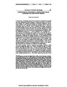
(a)
(b)
ij
ij ij
ij
αij
Lij
static loading surface, fs=0 bounding surface, F=0
ij
Lij ij
αij
relocated static loading surface, fs=0
bounding surface, F=0
Fig. 2. Schematic illustration of (a) initiation of stress reversal and (b) relocation of the static loading surface upon attaining a positive loading index
32
Shi, April 30, 2018
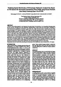
q
(ps, qs)
(p , q )
(p, q) (p, q) p0
p0/b
p
fs=0 F=0 Fig. 3. Schematic illustration of an isotropic bounding surface, static loading surface and associated radial mapping rule based on a projection center fixed at the origin of stress space
33
Shi, April 30, 2018
100
100
rate−independent model rate−dependent model: axial strain rate 0.1%/hr rate−dependent model: axial strain rate 5%/hr
80 deviatoric stress q (kPa)
deviatoric stress q (kPa)
80 critical state line
60 initial bounding surface
40
20
60
40
20 (a)
(b)
0 0
20 40 60 80 effective mean normal stress p (kPa)
0
100
0
0.02
0.04 0.06 axial strain εa (m/m)
0.08
0.1
Fig. 4. Undrained triaxal compression tests simulated by the rate-independent bounding surface model and the corresponding rate-dependent model under different loading rates: (a) effective stress path and (b) stress-strain response
34
Shi, April 30, 2018
60
60
initial bounding surface
40 deviatoric stress q (kPa)
deviatoric stress q (kPa)
40
rate−independent model rate−dependent model: frequency 1E−5 Hz rate−dependent model: frequency 1E−3 Hz
20 0 −20 −40
20 0 −20 −40
(a)
(b)
−60 0
20 40 60 80 100 effective mean normal stress p (kPa)
−60 −0.006 −0.004 −0.002 0 0.002 axial strain εa (m/m)
120
0.004
0.006
Fig. 5. Undrained cyclic loading tests simulated by the rate-independent bounding surface model and the corresponding rate-dependent model under different loading rates: (a) effective stress path and (b) stress-strain response
35
Shi, April 30, 2018
70
critical state line
60 deviatoric stress q (kPa)
60 deviatoric stress q (kPa)
70
axial strain rate 0.1%/hr axial strain rate 5%/hr axial strain rate 10%/hr step−wise changes of strain rates
50 40 30 20
50
initial bounding surface
40 30 20 purely elastic response
10
10
(a)
0 0
0.02
0.04 0.06 axial strain εa (m/m)
0.08
(b)
0
0.1
0
10 20 30 40 50 60 effective mean normal stress p (kPa)
70
Fig. 6. Model simulations of undrained triaxial compression tests on OC clays with variable strain rates: (a) stress-strain response and (b) effective stress path
36
Shi, April 30, 2018
0
0.02 volumetric strain εv (m/m)
yielding
creep
0.04
stress relaxation
0.06
0.08
0.1
volumetric strain rate 0.1%/hr volumetric strain rate 50%/hr volumetric strain rate 100%/hr constant strain rate with creep and stress relaxation
0.12 10
100 effective mean normal stress p (kPa)
1000
Fig. 7. Model simulations of isotropic compression tests with variable strain rates
37
Shi, April 30, 2018
volumetric strain εv (m/m)
0
0.001
0.002 Cα 1 p
0.003
0.004
p0=100 kPa
p=50 kPa (OCR=2) p=75 kPa, (OCR=1.33) p=100 kPa, (OCR=1)
1
10
100
1000
time (s) Fig. 8. Model simulations of secondary compression on soils with varying OCR
38
Shi, April 30, 2018
350
300
300 excess pore pressure Ue (kPa)
deviatoric stress q (kPa)
350
250 200 150 100 50
experiment:axial strain rate 0.15%/hr axial strain rate 1.5%/hr axial strain rate 15%/hr simulation:axial strain rate 0.15%/hr axial strain rate 1.5%/hr axial strain rate 15%/hr
(a)
0 0
2
4
6 8 10 axial strain εa (%)
12
250 200 150 100 50
(b)
0 14
0
2
4
6 8 10 axial strain εa (%)
12
14
Fig. 9. Comparison between experimental observations and model simulations for undrained triaxial compression tests on HKM clay (OCR=1) with different strain rates: (a) stress-strain response and (b) excess pore pressure-strain response
39
Shi, April 30, 2018
300
100
excess pore pressure Ue (kPa)
deviatoric stress q (kPa)
250 200 150 100 experiment:axial strain rate 0.15%/hr axial strain rate 1.5%/hr axial strain rate 15%/hr simulation:axial strain rate 0.15%/hr axial strain rate 1.5%/hr axial strain rate 15%/hr
50 (a) 0 0
2
4
6 8 10 axial strain εa (%)
12
50
0
−50 (b) −100
14
0
2
4
6 8 10 axial strain εa (%)
12
14
Fig. 10. Comparison between experimental observations and model simulations for undrained triaxial compression tests on HKM clay (OCR=4) with different strain rates: (a) stress-strain response and (b) excess pore pressure-strain response
40
Shi, April 30, 2018
450
100
excess pore pressure Ue (kPa)
deviatoric stress q (kPa)
400 350 300 250 200 150 experiment:axial strain rate 0.15%/hr axial strain rate 1.5%/hr axial strain rate 15%/hr simulation:axial strain rate 0.15%/hr axial strain rate 1.5%/hr axial strain rate 15%/hr
100 50
(a)
0 0
2
4
6 8 10 axial strain εa (%)
12
50
0
−50
−100 (b) −150
14
0
2
4
6 8 10 axial strain εa (%)
12
14
Fig. 11. Comparison between experimental observations and model simulations for undrained triaxial compression tests on HKM clay (OCR=8) with different strain rates: (a) stress-strain response and (b) excess pore pressure-strain response
41
Shi, April 30, 2018