Proceedings of the Stockholm Music Acoustics Conference, August 6-9, 2003 (SMAC 03), Stockholm, Sweden
BOWED STRING PHYSICAL MODEL VALIDATION THROUGH USE OF A BOW CONTROLLER AND EXAMINATION OF BOW STROKES Stefania Serafin
Diana Young
CCRMA, Department of Music Stanford University, Stanford, CA, USA
[email protected]
MIT, Media Lab, Cambridge, MA, USA
[email protected]
with a stronger focus on performance issues rather than acoustical validation was proposed in [5]. In this research the combination of the input parameters of a bowed string physical model was used to reproduce different bow strokes such as detach´e, legato and spiccato. Although the goal was to reproduce a particular sound specific to a certain performer’s gesture, no real-time input controller was used. Definitions of playability more related to performance issues are described in [6]. In this paper we are interested in exploring the possibility of reproducing traditional bowing techniques using a bow controller that behaves in a manner as closely related to that of a traditional violin bow as possible. This allows us to validate both the model and the controller by comparing it to the behavior of the traditional instrument. We therefore used a real-time bowed string physical model and a wireless bow controller to reproduce the bow strokes that are most fundamental to the right hand technique of an accomplished bowed string player, such as legato, detach´e staccato, spiccato, and balzato. We discuss the integration of the two components of these experiments and illustrate how the bow controller is used to control the physical model of the violin in order to faithfully reproduce these strokes. Moreover, we compare the range of input parameters that determine these strokes in the model with the values for these parameters measured on real violins, showing how synthetic instruments may present the same playability regions as real instruments. The ultimate goal of this research is to create a bowed string instrument able to reproduce the behavior of a traditional instrument as well as to create extended performance techniques for bowed string players. In the following section the bowed string physical model used in the simulations is described.
ABSTRACT Combining a physical model with a bow controller, we propose a technique to validate bow strokes in a virtual instrument. 1. INTRODUCTION Bowed string physical models have achieved a level of completeness that allows their performance to be favorably compared to that of their real instrument counterparts. These comparisons are facilitated by the use of refined bow controllers that detect all the subtle changes in motion and force that are experienced by a bow while in contact with a string and give expressive playing its characteristic sound. In the bowed strings’ literature, research on playability has focused both on aspects related to musical acoustics and to musical controllers. In these different domains the word playability has different definitions. For example, according to Jim Woodhouse [1], playability of virtual instruments means that the acoustical analysis of the waveforms produced by the model fall within the region of the multidimensional space given by the parameters of the model. This is the region where good tone is obtained. In the case of the bowed string, good tone refers to the Helmholtz motion, i.e. the ideal motion of a bowed string that each player is trying to achieve. The Helmholtz motion is given by an alternation of stick-slipstick-slip, in which the string sticks to the bow hair for the longest part of its period, slipping just once. Experiments show that simulated bowed strings have the same playability as real bowed strings as calculated by Schelleng [2]. Further experiments also show that the playability of virtual bowed strings increases when accurate friction models that account for the thermodynamical properties of rosin are taken into account [3]. In these experiments, in fact, the input parameters that drive the bowed string model corresponding to the right hand of the player are kept constant for each simulation. This is a situation that is clearly not the same as that which occurs in violin performances. As in performance it is the continuous evolution of the input parameters that constitute the nuance that are the characteristics of an expressive performance. In order to address this issue, Askenfelt [4] studied the contribution of bowing parameters in different bow strokes, trying to determine the physical limits of the input parameters in order to achieve a specific stroke. He determined the maximal duration of the pre-Helmholtz attack allowed in order to judge a particular stroke as acceptable. The previous definition of playability is the one we are interested on examining in this paper. Similar work
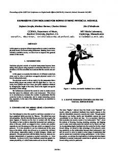
2. A BOWED STRING PHYSICAL MODEL We built a bowed string physical model that combines waveguide synthesis [7] with latest results on bowed string interaction modeling [8]. A schematic representation of the model is shown in Figure 1. In this model, the bow excites the string in a finite number of points, which represent the bow width. The frictional interaction between the bow and the string is modeled considering the thermodynamical properties of rosin, using the so-called plastic model proposed in [9], given by: µ=
Aky (T ) sgn(v) N
(1)
where A is the contact area between the bow and the string, N is
99
Proceedings of the Stockholm Music Acoustics Conference, August 6-9, 2003 (SMAC 03), Stockholm, Sweden NUT TRAVELING WAVES
the normal load, and ky (T ) is the shear yield stress as a function of temperature T . The temperature T of the shearing rosin layer can be estimated from the current sliding velocity v by passing it through an appropriate linear filter [9]. The bow width is modeled by discretizing the region of the string in contact with the bow using finite differences and calculating the coupling between the waves propagating along the string and the frictional interaction between the bow and the string at each point. Once the velocity of the string at the contact point has been calculated, the waves propagating along the string are modeled using digital waveguides. More precisely, transversal and torsional waves propagating toward the bridge and the fingerboard are modeled as pairs of one dimensional digital waveguides. The outgoing velocity at the bridge is filtered through the body’s resonances and corresponds to the output waveforms perceived by the listener. A preliminary version of this model has been described in [3]. The block diagram structure of the complete bowed string physical model is shown in Figure 2. In it delay lines correspond to traveling waves propagating from the bow point to the bridge and the nut; LP and AP represent respectively the lowpass filters that simulate losses and the allpass filters that simulate dispersion. The input parameters of the model corresponding to the right hand of the player are bow position relative to the bridge (normalized between 0 and 1, where 0 corresponds to the bridge, 1 corresponds to the nut, 0.5 corresponds to the middle of the string), bow pressure, bow velocity, and amount of bow hair in contact with the string. The model has been implemented as an external object in the Max/MSP environment.
BRIDGE TRAVELING WAVES
DELAY
DELAY
LP
AP
BOW−STRING
−1 DELAY
INTERACTION
DELAY
v−vb
DELAY f
TRASVERSAL WAVES
DELAY TORSIONAL WAVES
−1 DELAY
DELAY
Figure 2: Refined block diagram structure of the bowed string physical model used in the simulations.
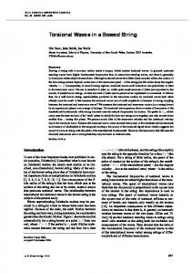
Figure 3: Data flow for the violin controller.
The system is comprised of an electric field sensor for measuring bow position (tip-frog / bow-bridge distance), commercial accelerometers for detecting 3D acceleration, and foil strain gauges for measuring the strain in the bow stick proportional to normal force on the string and the orthogonal force corresponding to flexion toward and away from the scroll. From these sensors, the parameters of bow velocity, bow-bridge distance, downward force, and bow width (using tilt information provided by the accelerometers and the second strain sensor) may be isolated from bowing gestures and used as input to the physical model. The implementation of the measurement system is minimal and maintains the playability of the interface in most scenarios. Though somewhat heavier than usual (almost 30g heavier, including battery), the resulting bow has a reasonable balance point and remains wireless. The microcontroller, battery, RF transmitter, and accelerometers are housed on an electronics board mounted on the frog, while the strain sensors are mounted directly to the bow stick around the midpoint of the bow. The acceleration and strain data is transmitted wirelessly to a bay station board. The bow board also sends two square wave signals to either end of a resistive strip that runs the length of the bow stick, acting as an antenna for the position measurement. The resultant signal is received by an antenna mounted behind the bridge of the violin, and this signal is connected via a cable to a small bay station board that determines the different amplitudes of the two received signals. The position information is then combined with the acceleration and strain data stream and output through a serial bus to the computer running the physical model. The compactness of this gesture measurement system allows for an easy test setup in a laboratory or performance environment.
Figure 1: Simplified structure of the bowed string physical model used in the simulation.
3. A BOW CONTROLLER The bow controller used in these experiments is a commercial carbon fiber bow, adapted by adding a custom measurement system.
100
Proceedings of the Stockholm Music Acoustics Conference, August 6-9, 2003 (SMAC 03), Stockholm, Sweden Using the bow controller to play a single string on the test violin, we were able to compare the sound produced by the model with that of the test violin. We were able to quickly produce sonorities from the model that sounded appropriate for the amount of pressure we applied to the bow. Interestingly, the model produced sounds that seemed perceptually correct for long sustained strokes as well as for short strokes with sharp attacks and decays.
For a detailed description of the bow controller, see [10]. 4. EXPERIMENTAL SETUP In these experiments we used a Macintosh G4 computer to run the Max/MSP implementation of the bowed string physical model. The gestural data from the bow controller was connected via a serial/USB converter to a USB port of the computer. The antenna used for the measurement of bow position was mounted behind the bridge of an electric violin (Jensen). This violin was chosen for these tests for ease of audio recording, as well as the ability to play the audio produced by the model and the unamplified violin sound together. Recordings of both the violin audio and the bow controller data were made simultaneously within the Max/MSP environment. The gesture data was then used to drive the physical model, which produced waveforms that were also recorded. This setup was simple enough to allow fast and easy recording and testing, and was used to reproduce some of the bow strokes that are fundamental to the right hand technique of an accomplished bowed string player, such as legato, detach´e, and balzato. The waveforms of the violin were then qualitatively compared to those produced by the model using both time and spectral domain evaluation and perceptual evaluation. The experimental setup used is shown in Figure 4.
4.2. Adding Velocity and Bow-Bridge Distance Next we added the bow velocity and bow-bridge distance controls by using the data from the bow position sensor. By taking the data values corresponding to the tip and the frog, the transverse bow position was determined, and from this the velocity value was derived. The bow-bridge distance was taken as the sum of the tip and the frog values. We were able to change the sound of the tones produced by the model by adjusting bow pressure, speed, bow-bridge distance, and by simply changing the bow direction. As the sound of the test violin offered an easy comparison to the model, we experimented by playing two open strings (of the test violin) while controlling a single tone of the model tuned to different intervals above and below the higher string. Playing the small duet between real and virtual violins we were able to make small adjustments in the mappings so that the timbers sounded as though they were all three emanating from the test violin. 5. COMPLETE MAPPING In order to build an expressive virtual musical instrument, the capture of the gesture of the performance is as important as the manner in which the mapping of gestural data onto synthesis parameters is done. In the case of physical modeling synthesis, a one-to-one mapping approach of control values to synthesis parameters makes sense due to the fact that the relation between gesture input and sound production is often hard-coded inside the synthesis model [?]. Because both the physical model and the bow controller are developed according to physical input and output parameters, the complete mapping between the two is straightforward. Figure 5 shows how all the data sent by the bow controller were mapped to the input parameters of the physical model. Downward bow force of the controller is directly mapped into bow force in the physical model. Bow velocity and bow-bridge distance were captured by measuring the horizontal and vertical position of the bow respectively. Moreover, lateral strain sensors were mapped onto the amount of bow hair in contact with the bow.
Max/MSP
Figure 4: Setup used for the experiments. 5.1. Bow strokes As mentioned in the previous paragraph, the evaluation of the bow strokes using the experimental setup was done by comparing the output of the electric violin to the output of the physical model, using the same input parameters. This evaluation was first performed by comparing the shape of the time domain and frequency domain waveforms produced by the two instruments. This evaluation, however, did not seem very effective: not surprisingly, waveforms with quite different shapes in some cases turned out to sound similar. Inspection of waveforms alone was not sufficient to determine the similarity between sounds. We therefore started performing
4.1. Playing with Downward Force We began the integration of the bow controller hardware with the software model by addressing one input parameter at a time. In the first trial we used the downward strain sensor to control the downward force parameter for the bowed string model. With the model parameters of bow-bridge distance, bow velocity, bow width, and frequency held constant, we varied the downward force between 0 and 5 N. Other than setting a threshold appropriate for the sensor range, it was unnecessary to perform any adjustments to this mapping.
101
Proceedings of the Stockholm Music Acoustics Conference, August 6-9, 2003 (SMAC 03), Stockholm, Sweden [8] R. Pitteroff, “Mechanics of the contact area between a violin bow and a string. part i:reflection and transmission behaviour. part ii: Simulating the bowed string. part iii: Parameter dependance,” in Acustica-Acta Acustica, 1998, pp. 543–562. [9] Jonathan H. Smith and James Woodhouse, “The tribology of rosin.,” J. Mech Phys.Solids, vol. 48, pp. 1633–1681. [10] Diana Young, “The hyperbow controller: Real-time dynamics measurement of violin performance,” in Proc. NIME, 2002.
Figure 5: Final mappings of the bow controller to the bowed string physical model.
listening tests to evaluate the accurateness of the overall setup. 6. CONCLUSIONS We proposed the combination of a bowed string physical model and a bow controller to examine how different bow strokes can be achieved in a virtual bowed string instruments. Preliminary experiments show that the bow strokes that a beginner’s violin player learns after few years of practice are easily reproduced. More accurate listening tests and comparisons between all the variations of input parameters and bow strokes need to be tested in order to fully validate the playability of our instrument. 7. REFERENCES [1] James Woodhouse, “On the playability of violins. Part I: Reflection functions. Part II: Minimum bow force and transients,” Acustica, vol. 78, pp. 125–136,137–153, 1993. [2] John C. Schelleng, “The bowed string and the player,” Journal of the Acoustical Society of America, vol. 53, no. 1, pp. 26–41, Jan. 1973. [3] Stefania Serafin, Julius O. Smith, III, and Jim Woodhouse, “An investigation of the impact of torsion waves and friction characteristics on the playability of virtual bowed strings,” New York, Oct. 1999, IEEE Press. [4] Anders Askenfelt, “Measurement of the bowing parameters in violin playing,” Journal of the Acoustical Society of America, vol. 86, no. 2, pp. 503–516, August 1989. [5] David Jaffe and Julius Smith, “Performance expression in commuted waveguide synthesis of bowed strings,” in Proc. International Computer Music Conference. ICMA, 1995, pp. 343–346. [6] D. Young and S. Serafin, “Playability evaluation of a virtual bowed string instrument,” in Proc. NIME, Montreal, CA, 2003. [7] Julius O. Smith, “Physical modeling using digital waveguides,” Computer Music Journal, vol. 16, no. 4, pp. 74–91, Winter 1992.
102