BoxRouter: A New Global Router Based on Box ... - IEEE Xplore

This article has been accepted for publication in a future issue of this journal, but has not been fully edited. Content may change prior to final publication.

BoxRouter: A New Global Router Based on Box Expansion and Progressive ILP Minsik Cho and David Z. Pan

Abstract— In this paper, we propose a new global router, BoxRouter, powered by the concept of box expansion, progressive integer linear programming (ILP), and adaptive maze routing. BoxRouter first uses a simple PreRouting strategy to predict and capture the most congested region with high fidelity, compared to the final routing. Based on progressive box expansion initiated from the most congested region, BoxRouting is performed with progressive ILP and adaptive maze routing. Our progressive ILP is shown to be much more efficient than traditional ILP in terms of speed and quality, and the adaptive maze routing based on multi-source multi-target with bridge model is effective in minimizing the congestion and wirelength. It is followed by an effective PostRouting step which reroutes without ripup to enhance the routing solution further and obtain smooth trade-off between wirelength and routability. Our experimental results show that BoxRouter significantly outperforms the stateof-the-art published global routers, e.g., 91% better routability than [1] (with 14% less wirelength and 3.3x speedup), 79% better routability than [2] (with similar wirelength and 2x speedup), 4.2% less wirelength and 16x speedup than [3] (with similar routability). Additional enhancement in box expansion and PostRouting further improves the result with similar wirelength, but much better routability than the latest work in global routing [4], [5]. Index Terms— Global routing, physical design, congestion, routability, integer linear programming (ILP), rectilinear minimum Steiner tree

I. I NTRODUCTION Routing is a key stage for VLSI physical design. Aggressive technology scaling has led to much smaller/faster devices, but more resistive interconnects and larger coupling capacitance. Since routing directly determines interconnects (wirelength, routability/congestion, and so on) and the overall VLSI system performance [6]–[8], it plays a critical role in the deep submicron design closure. For nanometer interconnects, the manufacturability and variability issues such as antenna effect, copper chemical-mechanical polishing (CMP), subwavelength printability, and yield loss due to random defects are becoming growing concern and shown to be directly impacted by wire embedding [8]–[15]. Thus, routing plays a major role in terms of the manufacturing closure as well. This work is supported in part by SRC under contracts 2005-TJ-1321 and 2005-TJ-1362, IBM Faculty Award, Fujitsu, Sun, and equipment donations from Intel. M. Cho and D. Z. Pan are with Electrical & Computer Engineering Department, The University of Texas at Austin, Austin, TX 78712 USA (email: [email protected];[email protected]). Copyright (c) 2007 IEEE. Personal use of this material is permitted. However, permission to use this material for any other purposes must be obtained from the IEEE by sending an email to [email protected].

In general, routing consists of two steps, global routing and detailed routing. While detailed routing finalizes the exact DRC-compatible pin-to-pin connections, the global routing, as its name implies, is the routing stage that plans the approximate routing path of each net to reduce the complexity of routing task and guide the detailed router [16]. Thus, it has significant impact on the overall wirelength, routability, and timing [16], [17]. Furthermore, it is also the key stage for optimizing the wire density distribution to improve the overall manufacturability (e.g., less post-CMP topography variation, less copper erosion/dishing, and less optical interference for better printability [10]–[13]) and yield (e.g., smaller critical area [14], [15]). The importance of global routing in VLSI design flow has led to many works in predicting and estimating routing congestion, and designing global routers. Probability based congestion prediction for global routing is studied in [18]–[21], and global router based congestion estimation is researched in [22], [23] for early wirelength estimation. Within the scope of over-the-cell global routing model [2], Burstein et al. [24] proposed a hierarchical approach to speed up integer programming formulation for global routing, and Kastner [25] proposed a pattern-based global routing. Raja et al. [2] presented Chi dispersion router based on linear cost function as well as predicted congestion map, and showed better results than [25]. The multicommodity flow-based global router by Albrecht [3] showed good results and was used in industry, but at the expense of computational effort. Fast global router [4], [26], [27] can feed more accurate interconnect information (such as wirelength and congestion) back to placement or other early physical synthesis engines for better design convergence and tighter integration. In this paper, a new routability-driven global router, namely BoxRouter is proposed. BoxRouter first performs a very fast yet effective PreRouting to identify the most congested regions or boxes. Then, it progressively expands the routing box, and performs routing within each expanded box (BoxRouting), until the entire circuit is covered, i.e., all the wires are routed. Efficient progressive ILP is formulated with adaptive maze routing, and effective PostRouting follows BoxRouting for further enhancement. The major contributions of this paper include the following. • We propose a new ILP formulation which is significantly faster and more scalable than the traditional formulation in [3], [28], which makes it practical to apply ILP to solve VLSI routing. • We observe that a simple PreRouting step can capture the overall congestion, and improve runtime. • We propose the key BoxRouting idea which efficiently


utilizes limited routing capacities based on box expansion initiated from the most congested region estimated by PreRouting. BoxRouting is efficient in terms of routability as the wires in the more congested region are routed before those in the less congested region. • We propose an efficient progressive integer linear programming (ILP) for BoxRouting. In our progressive ILP, only wires between two successive boxes are routed with L-shape patterns. Thus even with ILP, our runtime is still much faster than existing global routers [2], [3], [25]. • We propose an adaptive maze routing based on multisource multi-target with bridge model. Our adaptive maze routing uses different routing strategies inside and outside the box such that routability can be maximized with minimum wirelength increase. • We propose an effective PostRouting step which reroutes wires from the most congested region without rip-up. It is more efficient than the conventional rip-up & route. It also provides smooth trade-off between wirelength and routability with only a simple parameter. BoxRouter achieves much better results on the standard ISPD98 IBM benchmarks than [1]–[5], thus pushes the state-of-the-art considerably. Due to the fundamental importance of global routing in routability, timing, and manufacturability [29], we believe it shall have many applications/implications for nanometer designs. Preliminary work of BoxRouter is presented in [30]. The rest of the paper is organized as follows. In Section II, preliminaries are described. Previous works are surveyed in Section III. Comparison and evaluation of ILP formulations are presented in Section IV. In Section V, BoxRouter is proposed. Experimental results are discussed in Section VI. Section VII concludes this paper with future work. II. P RELIMINARIES A. Notations Table I lists the notations used throughout this paper. TABLE I T HE NOTATIONS IN THIS PAPER

vi eij mij cij

vertex / global routing cell i edge between vi and vj maximum routing capacity of eij available routing capacity of eij

C. Global Routing Metrics The key task of global router is to maximize the routability for successful detailed routing [27]. In addition, wirelength, runtime, and timing are other important metrics for global router. • Routability is usually the most important metric for global routing. It can be estimated by the number of overflows which indicates that routing demand exceeds the available routing capacity [25], [27]. In Fig. 1, the number of overflow between vA and vB is one, as there are four routed nets, but mAB = 3. Formal definition of overflow can be found in [25]. • Wirelength is an important metric for placement as well as routing. But, it is less important compared to routability, as most wires are routed with shortest distances, thus the total wirelength is in general not too far away from optimum for a reasonable global routing solution [27]. However, there can be huge difference in terms of routability between two different global routing solutions of similar wirelength. • Runtime is also an important consideration, as global routing links placement and detailed routing. A fast global router can feed proper interconnection information to higher level design flow for better design convergence [26]. • Other objectives such as timing and manufacturability are significant objectives as well. Since the focus of this paper is on the core global routing techniques, they are not explicitly considered in this work. However, our framework can be extended to handle them in the future. III. P REVIOUS W ORKS A. Congestion Prediction and Estimation Fast and accurate congestion prediction and estimation are essential techniques for reducing congestion in multiple stages of physical synthesis. For example, during placement, the cells can be inflated or the white space can be allocated in the congested region to reduce the congestion and enhance the routability [31], [32]. Recent study in congestion prediction includes a number of probabilistic approaches. Lou et al. [18] decompose a net into multiple two pin wires, then compute the probabilistic congestion for each G-cell based on the chance of having the two pin wire routed in the G-cell. While all possible detourfree paths are assumed with the same probability in [18], Westra et al. [20] only consider the simple L/Z shape routing

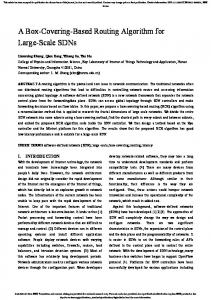
B. Global Routing Model The global routing problem can be modeled as a grid graph G(V, E), where each vertex vi represents a rectangular region of the chip, so called a global routing cell (G-cell), and an edge eij represents the boundary between vi and vj with a given maximum routing capacity mij . All the pins are assumed to be at the center of the corresponding G-cell. Fig. 1 shows how the chip can be abstracted into a grid graph where mAB = 3. A global routing is to find paths that connect the pins inside the G-cells through G(V, E) for every net.

A

A

B

3

B

G-cell

(a) real circuit with G-cells

(b) grid graph for routing

Fig. 1. A real circuit with netlists can be dissected into multiple grids which can be mapped into graph for global routing with routing capacity on an edge.


based on the observation that one or two-bend nets are dominant in the real designs. By empirically extracting the occurrence of L and Z shape routings from multiple real industrial designs, different probability weights are assigned to L and Z shapes routings. In [23], it is shown that fast global routing based congestion estimation can be more accurate than probabilistic congestion prediction, as probabilistic approach highly depends on tools or designs. However, global routing based congestion estimation is not exact neither. A recent paper [26] claims that congestion estimation can be different from global routing result, unless the same techniques and optimization parameters are applied in both congestion estimation and global routing.

V1

V2

V5

s V7

Integer linear programming (ILP) technique has been believed unacceptably slow for global routing in VLSI design, despite that it finds the global optimum for a given instance of problem. In this section, we propose a new ILP formulation for global routing, which is inherently different from the one in [3], [28], and discuss pros/cons of each formulation. In this work, to avoid any confusion, we call the traditional ILP as T-ILP and our new ILP as N-ILP. Both T-ILP and N-ILP are routability-driven, but they adopt different formulations, which make big difference in performance and scalability.

xb12

V4

wa3 a V8

wa1

V3

V5

V6

b s

xa11 V7

V9

V2

xb11 a xa21 xa31 a V8

V9

xa12

a

a

(a) decomposed net a,b

(b) routing candidates

V1

V2

V5

V6

xa31 a V8

s V7

xa12

a

V5

V6

b

xa11 V9

V3

xa21

xb12

V4

b s

V2

a

b

xa21

xb12

V4

V1

V3

a

b

B. Global Router

IV. P RACTICAL I NTEGER L INEAR P ROGRAMMING FOR G LOBAL ROUTING

V6

b

V7

Typical global router decomposes every net into a set of two pin wires by building minimum spanning tree or Steiner tree, then routes them by maze routing algorithm, followed by rip-up and reroute technique for further improvement. In [1], [25], Kastner et al. propose a simple pattern based routing rather than maze routing for fast runtime without incurring significant routing quality degradation. Hadsell et al. [2] take advantage of predicted congestion map to guide global router, and show considerable routing quality improvement over [1]. Congestion-aware Steiner tree in [4], [5], [26] reduces the runtime by increasing the number of nets routed by simple and fast pattern routing, and thus less relying on expensive maze routing. While the previous global routers [2], [25], [26] are mainly based on pattern routing, maze routing, or shortest path algorithm, Albrecht [3] formulates the global routing as multicommodity problem which can be solved by an approximation algorithm for fractional flow with randomized rounding. First, it repeats building a Rectilinear Minimum Steiner Tree (RMST) using maze routing in net-by-net manner. After all nets are routed in RMST, a set of G-cells above the given congestion threshold are selected, and all the nets on any of those G-cells are routed again by building new RMST. Two key advantages of such approach are that congestion can be evenly distributed over the chip and a small set of nets which are penalized by extreme detour will be discouraged. Overall, this algorithm shows good congestion reduction, but at a cost of high computational overhead.

b

wa2 wb1

V4

V1

V3

a

b

xa31 a V8

V9

a

(c) possible routing A

(d) possible routing B

Fig. 2. Example of ILP for global routing with two possible routing solutions is shown. Two routing solutions in (c) and (d) are valid w.r.t the given routing capacities, but different in terms of congestion distribution. The one in (c) achieves more uniform congestion distribution. T-ILP prefers routing (c) to routing (d), while N-ILP has no preference.

C

min : s.t :

xa11 , xa12 , xa21 , xa31 , xb11 , xb12 ∈ {0, 1} xa11 + xa12 = 1 xb11 + xb12 = 1 xa21 = 1, xa31 = 1

xa11

xa11 + xb12 ≤ C xa21 + xb11 ≤ C ≤ C, xa12 ≤ C, xa31 ≤ C xb11 ≤ C, xb12 ≤ C

Fig. 3.

T-ILP formulation for the example of Fig. 2 (b)

Before the main discussion, we describe Fig. 2 for clear explanation in the following sections. Fig. 2 (a) shows two unrouted nets a and b which are further decomposed into wires (See Section V-A): net a has three wires (wa1 , wa2 and wa3 ), and net b has one wire (wb1 ). For each wire, we can enumerate all the possible routing paths, but for simplicity we show only the paths in the minimum length and with minimum vias as in Fig. 2 (b). Each possible routing path is called a routing candidate of the given wire. In this example, we assume that the routing capacity is 2 for the all the edges (r12 = 2, r25 = 2, and so forth), thus both Fig. 2 (c) and (d) are routable solutions. A. T-ILP T-ILP minimizes the maximum congestion over all the edges. Fig. 3 is a T-ILP formulation of Fig. 2 (b) where a variable C is set to be larger than any congestion on any edge (i.e., the upper bound). The routing result after solving Fig. 3


min : s.t :

P

C xijk ∈ {0, 1}

P k:(i,j,k)∈N

(i,j,k)∈L(e)

Fig. 4.

max : ∀(i, j, k) ∈ N

xijk = 1

∀i, j

xijk ≤ C

∀e

General T-ILP formulation

is not Fig. 2 (d) but Fig. 2 (c), as Fig. 2 (d) has the maximum congestion 1.0 on e45 while Fig. 2 (c) has the maximum congestion 0.5. Let E be the set of edges in the grid (indexed by e), and let N be the set of all feasible routing candidates. Furthermore, let L(e) be the set of routing candidates crossing edge e. Suppose xijk is a binary variable set to 1 if the k-th routing candidate of wire j of net i is chosen. Then, Fig. 4 shows a general formulation of T-ILP. Note that the number of routing candidates must be kept small (L-shape or L/Z-shape path) due to practical limitations (e.g. memory). The advantages of T-ILP formulation include: • As it minimizes the maximum congestion (min-max formulation), it essentially tries to achieve more uniform congestion distribution. • The solution of T-ILP formulation always includes one routing candidate for each unrouted wire. Thus, it completes routing by itself, and does not need any additional step, unless there is any over-congested edge. Meanwhile, the drawbacks of T-ILP formulation include: • When C in Fig. 4 is larger than any me (the maximum routing capacity of the edge e), the number of overcongested edges will explode. It considers not the overall congestion but the maximum congestion. Therefore, as long as the congestion is smaller than C, it is possible to have many over-congested edges. • All the over-congested edges should be taken care of to meet congestion constraint (otherwise, it is unroutable by detailed router) by post-processing steps such as ripup&reroute. • The T-ILP cannot be efficiently solved with branchand-bound or branch-and-cut algorithms. This will be explained in Section IV-C.

max : 2xa11 + 2xa12 + xa21 + xa31 + 2xb11 + 2xb12 s.t : xa11 , xa12 , xa21 , xa31 , xb11 , xb12 ∈ {0, 1} xa11 + xa12 ≤ 1 xb11 + xb12 ≤ 1 xa21 ≤ 1, xa31 ≤ 1 xa11 + xb12 ≤ 2 xa21 + xb11 ≤ 2 xa11 ≤ 2, xa12 ≤ 2, xa31 ≤ 2 xb11 ≤ 2, xb12 ≤ 2 Fig. 5.

N-ILP formulation for the example of Fig. 2 (b)

s.t :

P

(i,j,k)∈N

xijk ∈ {0, 1} k:(i,j,k)∈N xijk ≤ 1

P

P

(i,j,k)∈L(e)

Fig. 6.

aijk · xijk

xijk ≤ ce

∀(i, j, k) ∈ N ∀i, j ∀e

General N-ILP formulation

B. N-ILP Our proposed N-ILP maximizes the weighted summation of the number of routed wires under the routing capacity constraint. Fig. 5 is a N-ILP formulation of Fig. 2 (b) where each routing candidate is weighted by its length in the objective. The result from Fig. 5 can be either Fig. 2 (c) or Fig. 2 (d), as N-ILP does not care about the maximum congestion, as long as there is no overflow. Fig. 6 shows the general formulation of N-ILP where aijk is the weight of the routing candidate xijk and the other notations are the same as in Fig. 4. Again, the number of routing candidates should be kept small (L-shape or L/Z-shape path). The advantages of N-ILP formulation include: • As each candidate xijk can have a different weight, other design objectives like timing can easily be incorporated. • Due to the hard constraint on routing capacity, the solution from N-ILP does not cause any over-congestion on any edge. • The N-ILP can be efficiently solved with branch-andbound or branch-and-cut algorithms. This will be explained in Section IV-C. However, the drawbacks of N-ILP formulation include: • The N-ILP may produce a biased routing solution in terms of congestion uniformness. For example, if there are two valid solutions with different congestion distributions, it may choose any of both depending on the solver regardless of congestion uniformness (See Fig. 2). • Different from T-ILP, it may not complete the routing. If the over-congested edge appears, it will give up routing some wires with smaller weight not to violate the hard routing capacity constraint. Thus, N-ILP requires an additional step for complete routing. C. T-ILP vs. N-ILP Based on the discussion in Section IV-A and IV-B, we compare both ILP formulations in two aspects: routability and runtime. 1) Routability: As mentioned earlier, both T-ILP and NILP maximize the routability, but in different manners: T-ILP minimizes the maximum congestion, but N-ILP maximizes the number of routed wires under the routing capacity constraint. This difference becomes highly distinct, depending on whether the design is under-congested or over-congested. • For under-congested designs, it is easy for T-ILP and N-ILP to satisfy the routing constraint. Therefore, T-ILP may be superior to N-ILP, as it can make more uniform


10 Normalized runtime (log scale)

•

congestion distribution which improves manufacturability and crosstalk noise. For over-congested designs, T-ILP may unnecessarily cause a lot of overflows, as it only cares about the maximum congestion. However, N-ILP itself does not cause any over-congested edges by leaving some wires unrouted. The overflows from T-ILP and the unrouted wires from N-ILP need to be picked up by the following maze routing.

10 10

4

2

1135 times

10 10 10

1

0

−1

Since, modern VLSI designs are highly congested in general, the advantage of T-ILP is quite trivial. 2) Runtime: For a given ILP solver, different ILP formulations may have different runtime complexity. An ILP problem is first solved as linear programming (LP), then branch based algorithm is applied to any fractional variable to find the integral optimal solution. We find that for the most widely used ILP solving algorithms, branch-and-bound or branch-andcut [33], [34], the N-ILP formulation can be solved much more efficiently than the T-ILP formulation for the same routing problem. For demonstration purpose, we prepare various routing problems in different problem sizes (in terms of the number of variables), then formulate them into both T-ILP and N-ILP. Fig. 7 shows the normalized runtime of each T-ILP and NILP formulation under typical computing environment (See Section VI) with GNU Linear Programming Kit (GLPK) 4.8 with all speedup options turned on. Note that we obtain very similar trend for various algorithms such as branch-and-bound and branch-and-cut with different cutting planes [34], [35]. It is clear that N-ILP is significantly faster than T-ILP, and such speedup becomes more significant for larger problem size, e.g., over 1100 times for some large cases. There are two theoretical explanations why N-ILP can be solved much faster than T-ILP. •

•

Since N-ILP is similar to a binary knapsack formulation, the solution after LP is a near feasible solution with almost all variables non-fractional [33], [36]. However, due to the min-max nature of the objective function, the variables in T-ILP have more incentive to remain fractional after LP as opposed to their counterparts in NILP. Consequently, the LP solution of T-ILP is much more fractional than that of N-ILP, resulting in more branches during branch-and-bound or branch-and-cut. The branch-and-bound or branch-and-cut techniques terminate in shorter time, if more nodes can be fathomed [33]. Unfortunately, the min-max nature of the objective function in T-ILP results in many near optimal solutions. Therefore, the corresponding nodes cannot be fathomed efficiently and the branch tree grows needlessly.

3) Summary: As discussed in Section IV-C.1 and IV-C.2, N-ILP is significantly faster than T-ILP, and the solution quality from N-ILP is similar to that from N-ILP for the overcongested design. Thus, N-ILP is expected to work better for the modern VLSI designs. Our proposed N-ILP is adopted in BoxRouter in Section V, in progressive manner with box expansion concept.

T−ILP N−ILP

3

0

0.5

1

1.5

2

2.5 3 Problem size

3.5

4

4.5

5 4

x 10

Fig. 7. Runtimes of T-ILP and N-ILP are compared. It shows that N-ILP is much faster and more scalable for larger problems than T-ILP.

V. B OX ROUTER In this section, we present our new global router, BoxRouter, which is based on congestion-initiated box expansion. BoxRouter progressively expands a box which initially covers the most congested region only, but finally covers the whole circuit. After every expansion, a circuit is divided into two sections, inside the box and outside the box. BoxRouter uses different routing strategies for each section to maximize routability and minimize wirelength. Consider Fig. 8 (a), where two wires (a and b) are inside the box, while the other wires (c and d) are not inside the box. The routing capacity inside the box is more precious to a and b than c and d for two reasons: • If a and b are not routed within the box, wirelength will increase due to detour. • c and d may have another viable routing path outside box which does not waste the routing capacity inside the box. Therefore, BoxRouter first routes as many wires inside the box as possible with N-ILP in Section IV-B, maximally utilizing the routing capacity inside the box. Then, for the wires which cannot be routed by N-ILP within the box (due to insufficient routing capacities), BoxRouter detours them by adaptive maze routing with the following two strategies: • Inside the box, use the routing capacities as much as possible (greedily), as the wires inside the box have priority over those outside the box. • Outside the box, use the routing capacities conservatively, as the wires outside the box may need them later for their viable routing paths.

c c b

a

Box Keep dense with greedy strategy

d b

a d

(a) motivation for BoxRouting Fig. 8.

The basic concept of BoxRouter

Keep uniform with conservative strategy (b) strategies of BoxRouting


Algorithm 1 PreRouting Input: A list of wires W 1: Sort each w in W by length in ascending order 2: for each w in W do 3: if w is flat then 4: Make w routed 5: OF = the number of updated overflows 6: if OF > 0 then 7: Make w unrouted 8: end if 9: end if 10: end for

Minimum Steiner Tree Net Decomposition PreRoute & Initial Box

BoxRoute

BoxRouter

Progressive ILP Routing Adaptive Maze Routing Box Expansion all wires routed?

N

Y PostRoute

Fig. 9. BoxRouter consists of three main steps: PreRouting, BoxRouting, and PostRouting. BoxRouting can be further composed of progressive ILP and adaptive maze routing.

Those two strategies keep the wire density of the circuit as in Fig. 8 (b), and make the wires detour the more congested region to maximize the routability with minimum wirelength overhead. The overall flow of BoxRouter is in Fig. 9, which will be explained in detail in the rest of this section. Section VA describes the preprocessing for BoxRouter. Section V-B illustrates PreRouting for congestion estimation and routing speedup. Section V-C explains BoxRouting, the main idea of BoxRouter which includes progressive ILP (PILP), adaptive maze routing (AMR), and box expansion. Finally, Section VD shows how PostRouting improves wirelength and routability further while controlling the trade-off between them.

(a) congestion after PreRouting

(b) congestion after BoxRouting

Fig. 11. Congestion estimations after PreRouting and BoxRouting are compared. It shows that simple PreRouting can effectively capture overall congestion as well as the most congested region.

routed. Routing each wire from a single net separately may have downside of loosing information on other wires, resulting in suboptimal routing. This issue is addressed in adaptive maze routing in Section V-C.2.

A. Steiner Tree and Net Decomposition

B. PreRouting and Initial Box

A net can be decomposed into two pin wires with Rectilinear Minimum Steiner Tree as shown in Fig. 10. In BoxRouter, Flute [37] and GeoSteiner [38], [39] are tested for Steiner tree construction, but Flute is finally adopted due to its small computational overhead. Note that different Steiner tree algorithms such as timing-driven or congestion-driven Steiner tree algorithms can be used in BoxRouter as well. A special wire which does not need a bend is called a flat wire [18]. For example, wire a-e, e-d, e-f and b-f in Fig. 10 (b) are flat wires, while wire f-c requires at least one bend to be routed. Each wire from a net becomes a single routing object. However, the net is finally routed, only if all the wires from a net are

PreRouting simply routes as many flat wires as possible via the shortest path without creating any overflow as in Algorithm 1. As bulk of nets are destined to be routed in simple patterns (L-shape or Z-shape) [20], [23], [25], PreRouting can improve the runtime without degrading the final solution. More importantly, if enough number of wires can be routed by PreRouting, the global congestion can be captured with reasonable accuracy. According to our experiments for the tested benchmarks, about 60% of the final wirelength on average can be routed with tiny computational overhead by PreRouting. Fig. 11, shows two congestion maps, one after PreRouting and the other one after BoxRouting where more congested area is brighter. It shows that congestion hotspots in Fig. 11 (b) can be predicted from Fig. 11 (a) by PreRouting. A box which encompasses the four G-cells in the most congested area will be created as shown in Fig. 12 (a) as a starting point of BoxRouting. Note that if there are two most congested areas, then the one closer to the center of the circuit is selected.

a

a wire a-e

d

wire e-d d

e wire e-f

b

b

net a-b-c-d (a) hypergraph for a net

c

wire b-f

f

wire f-c c

(b) wires after decomposition

Fig. 10. Net can be decomposed into two pin wires with Rectilinear Minimum Steiner Tree Construction.

C. BoxRouting In this subsection, BoxRouting will be explained with Fig. 12. BoxRouting consists of three steps, progressive integer linear programming routing, adaptive maze routing, and box expansion as in Fig. 9. Those three steps are repeated until the


a Box i

k

f

f

a c

b d

vA

h

b

f

xf1

xb1

h

k

d i

vC

c

xh1

xh2

h b

Box i

vB

f

xb2

h b

vD

i

(a) Initial box is created on the hotspot which

(b) Box i with wires which will be routed

is estimated by PreRouting.

by BoxRouting is shown.

(c) Wires within Box i will be routed by progressive ILP.

a Box i

k

f

f

b d

h

a k

a c

f

f

b d

k

k

a c

h

h

h h

h

c

d

i

i

a c

k b d

c

i

i

(e) Box i is expanded, and more wires are

is routed by adaptive maze routing.

enclosed by Box i+1.

c

i

(f) BoxRouting is performed with Box i+1.

BoxRouting example

max :xb1 + xb2 + xf 1 + xf 2 + xh1 + xh2

xb2 + xh2 ≤ cAC xb2 + xh2 ≤ cCD Progressive ILP formulation of Fig. 12 (c)

expanded box covers the whole circuit. Each of those steps are explained in the following subsections. 1) Progressive ILP Routing (PILP): We show in Section IV that N-ILP is more efficient than T-ILP for modern, typically over-congested VLSI design. Therefore, we use NILP formulation in PILP and further extend it by combining it with the box expansion concept. Assuming a box is expanded from the most congested region as in Fig. 12 (a), consider Fig. 12 (b), where wires within the box after i-th expansion (box i) are shown with squares (b, f and h), and the other wires are shown with circles. The already routed wires by either PreRouting or previous BoxRouting are simply shown as solid lines. Note that some flat wires like f, i and k could be remained unrouted

∀i ∈ Wbox

s.t :xi1 , xi2 ∈ {0, 1}

∀i ∈ Wbox

xi1 + xi2 ≤ 1 xi2 = 0 X xij ≤ ce

xf 1 + xf 2 ≤ 1 xf 2 = 0 xh1 + xh2 ≤ 1 xb1 + xf 1 + xh1 ≤ cAB xb1 + xh1 ≤ cBD

X

{xi1 + xi2 }

max :

s.t :xb1 , xb2 , xf 1 , xf 2 , xh1 , xh2 ∈ {0, 1} xb1 + xb2 ≤ 1

Fig. 13.

f

d

(d) Unrouted wire b after progressive ILP Fig. 12.

f

b

d

Box i+1 Box i

b

k

b

i

a

Box i+1 Box i

∀i ∈ Wbox ∀i ∈ Wbox ∩ Wf lat ∀e ∈ Wbox

e∈xi,j

Fig. 14.

General progressive ILP formulation

until BoxRouting, if PreRouting gives up routing them due to any overflow, or new Steiner points introduced by adaptive maze routing (AMR) (explained later in this section) convert a non-flat wire into a flat wire. For efficient routing as mentioned in the beginning of this section, only wires within the box will be routed by PILP and AMR. In Fig. 12 (c), the wires within the box are shown with G-cells (vA , vB , vC and vD ), and the corresponding PILP formulation for maximum routability is shown in Fig. 13. To minimize the number of vias, two L-shape routing candidates (xb1 , xb2 and xh1 , xh2 ) are considered for each wire in our PILP formulation, but only one routing candidate (xf 1 and xf 2 =0) is considered for flat wires. General PILP formulation is shown in Fig. 14, where ce is the available routing capacity on edge e (See Table I), Wbox is a set of unrouted wires within the current box, and Wf lat is a set of flat wires. Different from the hierarchical ILP [24], our PILP progressively routes a part of the circuit, which is covered by each expanding box. This box expansion limits the problem size


Algorithm 2 BoxRouting Input: A list of wires W in box B 1: Solve progressive ILP with W 2: for each w in W do 3: if w is unrouted then 4: Perform adaptive maze routing for w 5: end if 6: end for

Algorithm 3 Adaptive Maze Routing Cost for BoxRouting Input: G-cell Vx , Vy , Box B 1: Cost C = mxy − cxy 2: if exy is inside B and cxy > 0 then 3: C=1 4: end if Output: C

such that PILP which is NP-hard can be solved efficiently. Three advantages of our PILP can be summarized as follows: • Basic formulation is the same as N-ILP of Section IV-B, inheriting its advantages in runtime and scalability. • Even though the last box can cover the whole circuit, the PILP size remains tractable, as N-ILP is performed on the wires between two successive boxes like between Box i and Box i+1 in Fig. 12 (e). • As shown in Fig. 12 (e), the newer box always contains the older box. Consequently, the solution from the older PILP is reflected in the newer PILP formulation, providing smooth transition between two successive problems for high quality solution. Due to the limited routing capacity of each edge, some wires may not be routed with the above PILP. xi1 + xi2 ≤ 1 in Fig. 14 relaxes the routing constraint such that some wires may not be routed if the overflow occurs. For example, assuming mBD = mCD = 2 and xh1 = 1, the wire b cannot be routed with ILP (xb1 = xb2 = 0), as two prerouted wires on eCD , and one prerouted wire with the wire h (xh1 = 1) on eBD consume all the routing capacities. For this case, the wire b is routed by AMR as in Fig. 12 (d) with the routing cost from Algorithm 3. 2) Adaptive Maze Routing (AMR): Algorithm 3 returns a unit cost as long as eXY is inside box and still has available routing capacity (line 2, 3). Otherwise, it returns a cost inversely proportional to the available routing capacities (line 1). This cost function makes maze routing adaptively find the best routing path such that the shortest path inside the box for wirelength minimization, but the most idle path outside the box for routability maximization. Note that the resource outside the box should be used conservatively, as the wires outside the current box may need them later. If too big detour

c

a

path3 x

path2 x

y S

path1

T

b

path2 (a) by finding shorter path x-y

S

c b y path3

path1

T

a (b) by sharing routed path x-y

Fig. 15. Efficient multi-source multi-target maze routing examples are illustrated. More efficient alternative paths are found by considering multiple sources and targets.

is required to avoid small overflows, AMR may return a path with overflows for the least overall cost. For the maze router implementation, we propose a multisource multi-target with bridge (MMB) maze routing model for higher efficiency as illustrated in Fig. 15. Consider the example in Fig. 15 (a) where the source G-cell S and the target G-cell T are to be routed and the congestion is represented as shaded region. To avoid congestion, a simple maze routing can easily find the routing path path2 instead of path1. However, as the goal is to make S and T electrically connected, we can achieve electrical connection as well as shorter wirelength by alternatively routing x and y shown as path3. The other example in Fig. 15 (b) shows the case where the routing between b and c is detoured due to congestion. In this case, even though path1 is the shortest path between S and T without any congestion issue, the path S-x-y-T shown as path2 − path3 is the better routing path, because it shares and utilizes the existing routed path path3, resulting in the shorter total wirelength.

bridge group 1 S T

bridge group 2

source group

Fig. 16.

target group bridge group 3

Multi-source multi-target with bridge maze routing model

Aware of the above mentioned cases, the proposed multisource multi-target with bridge (MMB) based maze routing in Fig. 16 is implemented for AMR. The basic idea behind MMB is to make the maze router honor the existing partial routed paths of the net for shorter wirelength and less congestion. In detail, the proposed model is based on three different groups of G-cells as in Fig. 16. • Source group: a group of G-cells which are electrically connected to the source G-cell S. • Target group: a group of G-cells which are electrically connected to the target G-cell T . • Bridge group: multiple groups of G-cells on the partial routing paths which are connected to neither the source S nor the target T . Note that identifying each group of G-cells can be done with any graph traversal algorithm with trivial computational


Algorithm 4 Adaptive Maze Routing Input: Source s and target t of net N with box B 1: Find source group Gs of s 2: Find target group Gt of t 3: Find all bridge groups Gb1 , Gb2 , ... of N 4: A priority queue Q = φ 5: for each G-cell Vx in Gs do 6: Cost Tx of Vx = 0 7: Enqueue Vx into Q 8: end for 9: Best target G-cell Vb = φ, Tb = ∞ 10: while Q is not empty do 11: dequeue a G-cell Vx from Q 12: if Tx ≥ Tb then 13: break 14: end if 15: for each adjacent G-cell Vy of Vx do 16: Tn = Algorithm 3 (Vx , Vy , B) 17: Ty = Tx + Tn 18: if Vy ∈ Gt and Ty < Tb then 19: V b = V y , Tb = T y 20: else if Vy ∈ Gbi then 21: for each G-cell Vz in Gbi do 22: Tz = Ty 23: Enqueue Vz into Q 24: end for 25: else 26: Enqueue Vy into Q 27: end if 28: end for 29: end while 30: P = Backtrace the best path from Vb to any G-cell of Gs Output: P

overhead. There can be multiple bridge groups in case that many routed paths (from PreRouting or previous AMR) are not connected with each other. Flooding of the maze routing is started from the all the Gcells in the source group, and is terminated when any G-cell in the target group with the minimal cost is discovered. The flooding within a bridge group is free by treating one bridge group as a single virtual G-cell to encourage the utilization of the existing routed paths for shorter total wirelength. Details on AMR is in Algorithm 4. It should be noted that MMB based maze routing may change the initial Steiner tree structure according to the congestion updated during routing, and this may negatively affect the runtime as the maze router needs to search larger space for the optimal routing path. This runtime issue can be mitigated if the congestion-driven Steiner tree algorithm is adopted. Note that simple wirelength-driven Steiner tree algorithm is used in this work. 3) Box Expansion: After all the wires inside the box are routed either by PILP or AMR, the box i will be expanded to box i+1, and new wires (c, d and k) are encompassed by box i+1 as shown in Fig. 12 (e). The result after applying

BoxRouting (AMR after PILP) again is shown in Fig. 12 (f). The amount of increment during box expansion significantly affects the routing solution. As the box grows larger for every expansion with bigger increment, the runtime increases exponentially due to larger PILP problem size (more wires are added into the formulation due to larger expansion). But, the smaller overflow can be obtained, as the routing is performed more globally. There can be several heuristics to determine the increment such as constant increment size or dynamic increment size, but it is required to keep PILP problem size manageable. More discussion is presented in Section VI. After all wires are routed (the box becomes big enough to cover the whole circuit), PostRouting of Section V-D will follow BoxRouting. Each wire in the box is optimally routed by PILP, but the global optimality is not guaranteed as box expands. To certain extend, BoxRouting mimics the diffusion effect which was originally proposed for placement migration in [40]. By each BoxRouting step, all the wires in the more congested region (within the box) are routed first by PILP, then by AMR. This makes the wires outside the box detour the box, if necessary. Such box expansion and congestion spreading diffuses wires in a progressive and systematic manner. Our box expansion can be initiated from multiple regions, in case there are several congestion hotspots. This may lead to better congestion distribution as well as improved runtime. As the key idea behind box expansion is to diffuse wires from more congested regions to less congested regions, intuitively multiple box expansion has advantages. More importantly, multiple box expansion can be effectively performed on multiprocessor/distributed computing environment due to two reasons: a) most commercial ILP solvers itself support such computing environments; b) each PILP can be solved independently as long as boxes are not overlapped. However, several implementation issues such as where to begin (how to define congestion hotspot) and when to stop should be addressed with well-tuned heuristics. D. PostRouting (Reroute without Rip-up) As AMR in BoxRouting uses conservative strategy outside the box as in Algorithm 3 (finding the most idle routing path outside the box), it may create unnecessary detour and overflow. Thus, PostRouting simply reroutes wires to remove unnecessary overhead with box expansion initiated from the most congested region, as done in BoxRouting. In detail, a wire in the more congested region will be rerouted first, and such rerouted wire can release the routing capacity, as it may find the better routing path. Then, the surrounding wires can be rerouted with the released routing capacity, potentially reducing wirelength and overflow again. This chain reaction propagates from the most congested region to less congested regions along the box expansion. Consider the example in Fig. 17 where two wires x and y are routed around the Gcell Vz . Before the PostRouting (thus, during BoxRouting), the wire x detours Vz during AMR in Section V-C.2 due to high congestion in Vz in spite of the available routing capacity R. However, if R is still available after BoxRouting is finished, then there is no reason to leave R available at a cost of longer


x

TABLE II ISPD98 IBM BENCHMARKS FOR G LOBAL ROUTING

x

R

vz R

vz

x y

x

y

(a) routing before PostRouting

y

y

(b) routing after PostRouting

Fig. 17. Example of PostRouting is shown. In (a), a routing capacity R is not utilized by BoxRouting, as AMR finds less congested path. If R remains unused after BoxRouting is finished, it may be the reason for suboptimal routing path for a wire x. Thus, x can be rerouted by utilizing R, which shortens a wire y with the released routing capacity from x as well, as in (b).

wirelength. x can be rerouted through R to minimize the wirelength without causing any overflow. After x is rerouted, the wire y which is detoured during BoxRouting due to x can be rerouted as well using the routing capacity released after x is rerouted, thus reducing wirelength again. Algorithm 5 Maze Routing Cost for PostRouting Input: G-cell Vx , Vy , Param K 1: Cost C = K 2: if cxy > 0 then 3: C=1 4: end if Output: C AMR of Section V-C.2 is used again for PostRouting, but with a different routing cost function in Algorithm 5, where a user-defined parameter K is introduced. The parameter K controls the trade-off between wirelength and routability (overflow), by setting the cost of each overflow as K. Thus, higher K will discourage overflow at a cost of wirelength increase (more detours), but lower K will suppress detour at a cost of overflows. The effectiveness of parameter K is discussed in Section VI. Our PostRouting is more efficient than the widely used Ripup&Reroute (R&R), as PostRouting makes a wire voluntarily release a routing capacity (this happens, only when the solution improves) during its rerouting, while R&R deprives it from a wire in the congested region without guaranteeing any improvement. Although R&R and PostRouting target for less congestion, the approaches are different. While R&R rips up the already routed wires to secure routing capacity directly, PostRouting makes more routing capacity available indirectly by shortening the wirelength of each wire (wirelength is linearly proportional to the number of routing capacities in use). PostRouting is guaranteed to find the equal or better routing path for the given objective function, as the current routing path can always be found as the worst case routing path. Thus, the routing quality can be improved gradually by repeating PostRouting. VI. E XPERIMENTAL R ESULTS We implement BoxRouter in C++. All the experiments are performed on a 2.8 GHz Pentium-4 Linux machine with 2G RAM. Flute [37] with high accuracy option is used for Rectilinear Minimum Steiner Tree, and GNU Linear Programming

circuit routing graph lb.d a b c name cells nets wires grids v. cap h. cap wlen ibm01 12036 11507 28232 64x64 12 14 60142 ibm02 19062 18429 55649 80x64 22 34 165863 ibm03 21924 21621 45727 80x64 20 30 145678 ibm04 26346 26163 53487 96x64 20 23 162734 ibm05 28146 27777 94304 128x64 42 63 409709 ibm06 32185 33354 82541 128x64 20 33 275868 ibm07 44848 44394 109365 192x64 21 36 363537 ibm08 50691 47944 133353 192x64 21 32 402412 ibm09 51461 50393 128708 256x64 14 28 411260 ibm10 66948 64227 182010 256x64 27 40 574407 a the number of wires after net decomposition b vertical routing capacity c horizontal routing capacity d asymptotic lower bound wirelength [39] hereafter in this section

TABLE III P RE ROUTING IN B OX ROUTER FOR ISPD98 IBM BENCHMARKS

circuit name ibm01 ibm02 ibm03 ibm04 ibm05 ibm06 ibm07 ibm08 ibm09 ibm10 a

PreRouting lb. wlen pr. wlena 60142 40992 165863 109519 145678 85628 162734 94644 409709 240781 275868 172988 363537 210904 402412 243517 411260 240928 574407 336999 average prerouted wirelength

% 68.2 66.0 58.8 58.2 58.8 62.7 58.0 60.5 58.6 59.7 61.0

Kit (GLPK) 4.8 [34] is used as ILP solver. We use ISPD98 IBM benchmarks [1] for our experiments. Table II summarizes each ISPD98 IBM benchmark circuit and its corresponding grid graph model. The lower bound wirelength of each circuit is computed by the most accurate GeoSteiner 3.1 [37], [39]. Table III shows the routing completion percentage after PreRouting. On average, 61% of the lower bound wirelength can be routed after PreRouting which is enough to capture the overall congestion as well as the most congested region. Further, over 61% routing completion even before the main routing phase will improve the runtime. Fig. 18 shows the overflow and runtime by the amount of box increment (See Section V-C) for one benchmark. It clearly shows that with larger box increment, the overflow decreases, but the runtime increases exponentially. While the wirelength varies only by 0.11%, the overflow decreases by 30%, but the runtime increases by 500%. It indicates that with larger box increment during box expansion of BoxRouting, the solution quality can be improved at a cost of runtime. The effectiveness of parameter K (See Section V-D) is shown in Fig. 19. It shows that with larger K, overflow decreases exponentially, but wirelength increases logarithmically. We constantly find that overflow saturates faster than


1200

34.6

1000

34.4

Runtime (sec)

400

750 300 500

Overflow Runtime

Runtime (sec)

Overflow

350

34.2 34 33.8

250 250

200 0

5

10

15

20

25

30

35

33.6 0

5

10

0 45

40

15

K

20

25

30

20

25

30

(a) ibm02

Box Increment

96

Overflow and runtime change by box increment for ibm04

Runtime (sec)

Fig. 18.

5

x 10

600

1.8

Wire length

Overflow

400

Overflow Wire length 200

0 0

1.75

5

10

15

20

25

95.5 95 94.5 94 0

5

10

15

K (b) ibm10

Fig. 20.

Runtime change by Parameter K

TABLE IV R ESULTS FROM B OX ROUTER FOR ISPD98 IBM BENCHMARKS

30

K (a) ibm02 5

x 10

400

Overflow Wire length

5.9

Wire length

Overflow

600

200

circuit name lb.wlen ibm01 60142 ibm02 165863 ibm03 145678 ibm04 162734 ibm05 409709 ibm06 275868 ibm07 363537 ibm08 402412 ibm09 411260 ibm10 574407 a

0 0

5

10

15

20

25

5.85 30

K

b c

BoxRouter (K=10) wlena ovflb w.o(%)c 65029 166 8.1 177921 43 7.3 149466 20 2.6 171044 378 5.1 409747 0 0.0 281715 7 2.1 374910 83 3.1 408897 46 1.6 417599 8 1.5 590738 18 3.0 average 3.4 wirelength hereafter in this section overflow hereafter in this section wirelength overhead

BoxRouter (K=15) wlen ovfl w.o(%) 65193 126 8.4 179086 33 8.0 149879 9 2.9 171756 342 5.5 409747 0 0.0 282002 5 2.2 376247 81 3.5 409584 31 1.8 418023 4 1.6 591820 10 3.0 3.7

(b) ibm10 Fig. 19.

Routability and wirelength trade-off by Parameter K

wirelength, and the best trade-off occurs between K=10 to K=15 for all the tested benchmarks. Fig. 20 also shows the runtime is independent of parameter K. The runtime variations stdev ( average ) of ibm02 and ibm10 are only 0.7% and 0.5% respectively, while K varies from 1 to 30. Table IV shows the routing results by BoxRouter with K=10 and K=15, the best trade-off found in Fig. 19. It shows that BoxRouter has on average 3.4% and 3.7% wirelength overhead (regarding the lower bound wirelength) for K=10 and K=15 respectively, and provides high quality solutions for larger circuits with small overflows. Table VI compares the congestion-initiated box expansion with the random-initiated box expansion when K=15. It shows that the box expansion initiated from the most congested

region can improve the number of overflow by 33.1 % on average, proving that it is more effective than randomly initiated one in terms of congestion. For thorough comparison, we download two available global routers, Labyrinth 1.1 [1], [25] and Fengshui 5.1 (which has the newest implementation of the Chi dispersion router) [2], [41], and implement multicommodity flow-based global router [3] in C++ (the binary is not available from the author). Note that we use the same routine for Rectilinear Minimum Steiner Tree, congestion estimation, and maze routing for fair comparison in the multicommodity flow-based global router implementation. Although the results of Labyrinth and Fengshui are reported in [2], we reproduce the results due to the recent update in the benchmarks [1]. Table V shows the experimental results and comparison for Labyrinth and Fengshui, and Table VII for the multicommodity flow-based router. As there is a trade-off between


TABLE V C OMPARISON WITH L ABYRINTH 1.1 [25] AND F ENGSHUI 5.1 (Chi DISPERSION ) [2] FOR ISPD98 IBM BENCHMARKS

circuit name ibm01 ibm02 ibm03 ibm04 ibm05b ibm06 ibm07 ibm08 ibm09 ibm10 a b

Labyrinth wlen ovfl 76517 398 204734 492 185116 209 196920 882 420583 0 346137 834 449213 697 469666 665 481176 505 679606 588

1.1 cpu(s) 21.2 34.5 36.3 83.5 59.2 104.3 228.1 238.7 359.3 435.7

Fengshui 5.1 wlen ovfl cpu(s) 66006 189 15.1 178892 64 47.9 152392 10 35.2 173241 465 54.1 412197 0 104.8 289276 35 80.1 378994 309 122.2 415285 74 113.8 427556 52 125.1 599937 51 212.9

BoxRouter wlen ovfl cpu(s) 65588 102 8.3 178759 33 34.1 151299 0 16.9 173289 309 23.9 409747 0 49.5 282325 0 33.0 378876 53 50.9 415025 0 93.2 418615 0 63.9 593186 0 95.1 average

speedup hereafter in this section ibm05 is dropped from comparison hereafter in this section, as it is a trivial case.

TABLE VI I MPROVEMENTS ON THE RANDOMLY INITIATED BOX EXPANSION (K=15)

circuit name ibm01 ibm02 ibm03 ibm04 ibm05 ibm06 ibm07 ibm08 ibm09 ibm10 a

Imprv. on Labyrinth Imprv. on Fengshui wlen(%) ovfl(%) spd(x)a wlen(%) ovfl(%) spd(x)a 14.3 74.4 2.5 0.6 46.0 1.8 12.7 93.3 1.0 0.1 48.4 1.4 18.3 100 2.1 0.7 100 2.1 12.0 65.0 3.5 0.0 33.5 2.3 18.4 100 3.2 2.4 100 2.4 15.7 92.4 4.5 0.0 82.8 2.4 11.6 100 2.6 0.1 100 1.2 13.0 100 5.6 2.1 100 2.0 12.7 100 4.6 1.1 100 2.2 14.3 91.7 3.3 0.8 79.0 2.0

Random wlen 65089 178924 149895 171812 409744 282875 375584 409025 418131 592784

Init.a ovfl 171 55 15 395 0 9 115 58 7 19

Congestion Init. Imprv. wlen ovfl wlen(%) ovfl(%) 65193 126 -0.2 26.3 179086 33 -0.1 40.0 149879 9 0.0 40.0 171756 342 0.0 13.4 409747 0 0.0 0 282002 5 0.3 44.4 376247 81 -0.2 29.6 409584 31 -0.1 46.6 418023 4 0.0 42.9 591820 10 0.2 47.4 average 0.0 33.1 average of 10 random initiations from low congested regions

TABLE VII C OMPARISON WITH MULTICOMMODITY FLOW- BASED ROUTER [3] FOR ISPD98 IBM BENCHMARKS

a b

wirelength and routability, we choose the parameter K of BoxRouter of Table V with wirelength constraint such that wirelength from BoxRouter is as small as or smaller than those from Labyrinth and Fengshui for fair comparison. Regarding Table VII, we first carefully choose the parameters of the multicommodity flow-based router for each benchmark such that the best results are yielded within 25 phases (the maximum phase in [3]), then simulate ibm01, ibm02, ibm04 and ibm07 (circuits with non-zero overflow in Table V) again for BoxRouter without any constraint. As shown in Table V, BoxRouter outperforms Labyrinth and Fengshui by wide margin. In terms of wirelength and overflow, BoxRouter can reduce the wirelength by 14.3%, the overflow by 91.7% compared with Labyrinth, and improve the overflow by 79% with similar wirelength (actually 0.8% better) compared with Fengshui. Also, BoxRouter is 3.3x and 2.0x faster than Labyrinth and Fengshui respectively. Multicommodity flow-based router and BoxRouter show very comparable overflow as shown in Table VII. However, BoxRouter is on average 15.7x, up to 29x faster, and produces 4.2% shorter wirelength on average than multicommodity flow-based router. It implies that BoxRouter can provide high quality global routing solution with significantly less design turn-around time.

BoxRouter Imprv.a wlen ovfl cpu(s) wlen(%) spd(x) 67674 41 11.8 1.9 12.8 182268 2 35.7 4.3 13.9 151299 0 16.9 5.9 19.5 173778 249 31.4 1.6 10.4 409747 0 49.5 282325 0 33.0 4.9 28.9 394170 0 50.8 3.5 24.2 415025 0 93.2 3.5 9.3 418615 0 63.9 5.4 11.4 593186 0 95.1 6.5 11.2 average 4.2 15.7 overflow is not shown, as both are highly comparable. only one phase is required for ibm05, a trivial case.

circuit name ibm01 ibm02 ibm03 ibm04 ibm05 ibm06 ibm07 ibm08 ibm09 ibm10

Multicommodity wlen ovfl cpu(s) 68981 43 151.2 190418 3 494.5 160755 0 329.8 176610 225 326.6 410954 0 28.2b 296981 0 951.8 408510 0 1229.0 429913 0 865.7 442514 0 726.7 634247 0 1068.4

Figure. 21 shows pie chart for cputime break down averaged from all the benchmark circuits. PreRouting takes negligible amount of total cputime (1.4%), while routing over 60% of wires. BoxRouting which may be considered the slowest part of BoxRouter due to ILP takes about 25%, while PostRouting takes over 57%. This proves that the proposed PILP is significantly fast while providing high quality solution. On the other hand, PostRouting which is mainly the maze routing is the current bottleneck in runtime for BoxRouter. So far, all the results from BoxRouter are with constant

Fig. 21.

Pie chart for average cputime break down


TABLE VIII C OMPARISON WITH D P ROUTER [5] AND FAST ROUTE 2.0 [4] FOR ISPD98 IBM BENCHMARKS

circuit name ibm01 ibm02 ibm03 ibm04 ibm06 ibm07 ibm08 ibm09 ibm10 a b c

DpRouter FastRoute wlen ovfl cpu(s)a wlen ovfl 63857 125 2.4 68489 31 178261 3 3.8 178868 0 150663 0 0.8 150393 0 172608 165 14.7 175037 64 286025 14 4.0 284935 0 379133 99 6.9 375185 0 412308 56 11.5 411703 0 419199 47 5.9 424949 3 598460 46 9.7 595622 0

2.0 BoxRouter+ Imprv. on DpRouter Imprv. on FastRoute 2.0 cpu(s)a wlen ovfl cpu(s) pilpb rertc wlen(%) ovfl(%) spd(x) wlen(%) ovfl(%) spd(x) 4.5 67052 0 261.6 2 50 -5.0 100 -109.0 2.1 100 -58.1 3.5 174898 0 62.3 6 1 1.9 100 -16.4 2.2 -17.8 0.8 149949 0 43.0 6 1 0.5 -53.8 0.3 -53.8 14.3 178653 37 1791.8 13 100 -3.5 77.6 -121.9 -2.1 42.2 -125.3 3.9 282218 0 69.2 7 2 1.3 100 -17.3 1.0 -17.7 4.7 378933 0 889.5 11 30 0.1 100 -128.9 -1.0 -189.3 10.2 409337 0 262.9 13 4 0.7 100 -22.9 0.6 -25.8 5.5 418817 0 115.4 9 1 0.1 100 -19.6 1.4 100 -21.0 8.2 587742 0 142.0 17 1 1.8 100 -14.6 1.3 -17.3 average -0.2 97.2 -56.0 0.6 80.7 -58.5 scaled runtime based on the runtime of Fengshui 5.1 in [26] and in Table V the number of PILP solved with up to 10,000 wires the number of PostRouting repeat

size of box increment and single PostRouting. However, it is possible to alter the size of box increment dynamically, and repeat PostRouting for further improvement. Instead of having constant size of box increment, we fix the maximum number of wires for each PILP which can be found by empirically testing ILP solver. Consequently, box is kept expanded until it covers the given maximum number of wires. We call the improved BoxRouter as BoxRouter+ as shown in Table VIII, and compare BoxRouter+ with the latest global routers, DpRouter [5] and FastRoute 2.0 [4]. Also, it shows the number of PILP instances with 10,000 maximum wires, and the number of repeated PostRouting. Overall, BoxRouter+ shows significantly better routability than DpRouter and FastRoute 2.0 with comparable wirelength, and completes the most number of circuits. However, BoxRouter+ is slower than DpRouter and FastRoute 2.0. The main bottleneck in BoxRouter+ depends on the difficulty of each circuit. If a circuit is relatively easy, which requires only one or two iterations of PostRouting, the main runtime bottleneck is solving larger ILP instance. For harder circuits, it requires multiple iterations of PostRouting which makes it the bottleneck for runtime. However, considering that the real bottleneck in VLSI routing flow is detailed routing, better routability can compensate the runtime overhead, as it can result in significant speedup in detailed routing.

VII. C ONCLUSION In order to cope with the increasing impact of interconnect on system performance, we present an efficient global router, BoxRouter to maximize the routability with minimum wirelength. Experimental results show that BoxRouter outperforms the state-of-the-art publicly available global routers in terms of wirelength, routability, and runtime. As the BoxRouter is still in beta version, we believe that further improvement can be achieved with multiple box expansions, faster ILP solver and so on. Current implementation of BoxRouter is available at www.cerc.utexas.edu/utda. We plan to address timing, crosstalk, and manufacturability issues on the top of the BoxRouter framework.

VIII. ACKNOWLEDGMENT The authors would like to thank Prof. Patrick Madden from SUNY Binghamton and Dr. Christoph Albrecht from Cadence Berkeley Lab for helpful discussions, Ilyas Mohamed Iyoob in Dept. Operation Research in Univ. of Texas at Austin for the comparison of ILP formulations, and Kun Yuan and Katrina Lu in UTDA Lab in Univ. of Texas at Austin for proofreading. R EFERENCES [1] http://www.ece.ucsb.edu/∼kastner/labyrinth/. [2] R. T. Hadsell and P. H. Madden, “Improved Global Routing through Congestion Estimation,” in Proc. Design Automation Conf., June 2003. [3] C. Albrecht, “Global Routing by New Approximation Algorithms for Multicommodity Flow,” IEEE Trans. on Computer-Aided Design of Integrated Circuits and Systems, vol. 20, May 2001. [4] M. Pan and C. Chu, “Fastroute 2.0: A high-quality and efficient global router,” in Proc. Asia and South Pacific Design Automation Conf., 2007. [5] Z. Cao, T. Jing, J. Xiong, Y. Hu, L. He, and X. Hong, “DpRouter: A Fast and Accurate Dynamic-Pattern-Based Global Routing Algorithm,” in Proc. Asia and South Pacific Design Automation Conf., 2007. [6] J. Cong, “Challenges and opportunities for design innovations in nanometer technologies,” in SRC Design Science Concept Papers, 1997. [7] R. Kastner, E. Bozorgzadeh, and M. Sarrafzadeh, “An Exact Algorithm for Coupling-Free Routing,” in Proc. Int. Symp. on Physical Design, April 2001. [8] D. Wu, J. Hu, and R. Mahapatra, “Coupling Aware Timing Optimization and Antenna Avoidance in Layer Assignment,” in Proc. Int. Symp. on Physical Design, April 2005. [9] G. Xu, L. Huang, D. Z. Pan, and D. F. Wong, “Redundant-Via Enhanced Maze Routing for Yield Improvement,” in Proc. Asia and South Pacific Design Automation Conf., Jan 2005. [10] L. Huang and D. F. Wong, “Optical Proximity Correction (OPC)Friendly Maze Routing,” in Proc. Design Automation Conf., June 2004. [11] J. Mitra, P. Yu, and D. Z. Pan, “RADAR: RET-Aware Detailed Routing Using Fast Lithography Simulations,” in Proc. Design Automation Conf., June 2005. [12] R. Tian, D. F. Wong, and R. Boone, “Model-Based Dummy Feature Placement for Oxide Chemical-Mechanical Polishing Manufacturability,” IEEE Trans. on Computer-Aided Design of Integrated Circuits and Systems, vol. 20, 2001. [13] T. E. Gbondo-Tugbawa, “Chip-Scale Modeling of Pattern Dependencies in Copper Chemical Mechanical Polishing Process,” in Ph.D. Thesis, Massachusetts Institute of Technology, 2002. [14] K. Sy-Yen, “YOR: a yield-optimizing routing algorithm by minimizing critical areas and vias,” IEEE Trans. on Computer-Aided Design of Integrated Circuits and Systems, vol. 12, no. 9, Sep 1993. [15] A. Venkataraman, H. Chen, and I. Koren, “Yield Enhanced Routing for High-Performance VLSI Designs,” in Proc. of SPIE the Microelectronics Manufacturing Yield, Reliability and Failure Analysis, Oct 1997. [16] J. Hu and S. Sapatnekar, “A Survey On Multi-net Global Routing for Integrated Circuits,” Integration, the VLSI Journal, vol. 31, 2002.


[17] ——, “A Timing-Constrained Algorithm for Simultaneous Global Routing of Multiple Nets,” in Proc. Int. Conf. on Computer Aided Design, 2000. [18] J. Lou, S. Krishnamoorthy, and H. S. Sheng, “Estimating Routing Congestion using Probabilistic Analysis,” in Proc. Int. Symp. on Physical Design, 2001. [19] A. B. Kahng and X.Xu, “Accurate Pseudo-Constructive Wirelength and Congestion Estimation,” in Proc. System-Level Interconnect Prediction, April 2003. [20] J. Westra, C. Bartels, and P. Groeneveld, “Probabilistic Congestion Prediction,” in Proc. Int. Symp. on Physical Design, April 2004. [21] C. Sham and E. F. Y. Young, “Congestion Prediction in Early Stages,” in Proc. System-Level Interconnect Prediction, April 2005. [22] M. Wang and M. Sarrafzadeh, “Modeling and Minimization of Routing Congestion,” in Proc. Design Automation Conf., 2000. [23] J. Westra, C. Bartels, and P. Groeneveld, “Is Probabilistic Congestion Estimation Worthwhile?” in Proc. System-Level Interconnect Prediction, April 2005. [24] M. Burstein and R. Pelavin, “Hierarchical Global Wiring for Custom Chip Design,” IEEE Trans. on Computer-Aided Design of Integrated Circuits and Systems, vol. 2, no. 4, Oct 1983. [25] R. Kastner, E. Bozorgzadeh, and M. Sarrafzadeh, “Pattern Routing: Use and Theory for Increasing Predictability and Avoiding Coupling,” IEEE Trans. on Computer-Aided Design of Integrated Circuits and Systems, vol. 21, July 2002. [26] M. Pan and C. Chu, “Fastroute: A step to integrate global routing into placement,” in Proc. Int. Conf. on Computer Aided Design, 2006. [27] J. Westra, P. Groeneveld, T. Yan, and P. H. Madden, “Global Routing: Metrics, Benchmarks, and Tools,” in IEEE DATC Electronic Design Process, April 2005. [28] X. Yangand, R. Kastner, and M. Sarrafzadeh, “Congestion Reduction During Placement Based on Integer Programming,” in Proc. Int. Conf. on Computer Aided Design. [29] M. Cho, H. Xiang, R. Puri, and D. Z. Pan, “Wire Density Driven Global Routing for CMP Variation and Timing,” in Proc. Int. Conf. on Computer Aided Design, Nov 2006. [30] M. Cho and D. Z. Pan, “BoxRouter: A New Global Router Based on Box Expansion and Progressive ILP,” in Proc. Design Automation Conf., July 2006. [31] H. Ren, D. Z. Pan, C. Alpert, and P. Villarrubia, “Diffusion Based Placement Migration,” in Proc. Design Automation Conf., June 2005. [32] X. Yang, B.-K. Choi, and M. Sarrafzadeh, “Routability-driven white space allocation for fixed-die standard-cell placement,” April 2003. [33] L. A. Wolsey, “Integer programming,” in J. Wiley, 1998. [34] http://www.gnu.org/software/glpk/glpk.html/. [35] G. C. E. Balas, S. Ceria and N. Natraj, “Gomory Cuts Revisited,” in Operations Research Letters, vol. 19, no. 1, 1996. [36] A. Osyczka, “Multicriterion optimization in engineering - with fortran programs,” in Ellis Horwood, 1984. [37] C. C. N. Chu, “FLUTE: Fast Lookup Table Based Wirelength Estimation Technique,” in Proc. Int. Conf. on Computer Aided Design, 2004. [38] D. Warme, “Spanning Trees in Hypergraphs with Applications to Steiner Trees,” in Ph.D. Thesis,Computer Science Dept., The University of Virginia, April 1998. [39] http://www.diku.dk/geosteiner/. [40] H. Ren, D. Z. Pan, C. Alpert, and P. Villarrubia, “Diffusion Based Placement Migration,” in Proc. Design Automation Conf., 2005. [41] http://vlsicad.cs.binghamton.edu/.