Brain Tumor Segmentation Using a Fully Convolutional Neural Network with Conditional Random Fields Xiaomei Zhao1 , Yihong Wu1 , Guidong Song2 Zhenye Li3 Yong Fan4 and Yazhuo Zhang2,3,5,6 1
National Laboratory of Pattern Recognition,Institute of Automation, Chinese Academy of Sciences
[email protected];
[email protected] 2 Beijing Neurosurgical Institute, Capital Medical University 3 Department of Neurosurgery, Beijing Tiantan Hospital, Capital Medical University 4 Department of Radiology, Perelman School of Medicine, University of Pennsylvania 5 Beijing Institute for Brain Disorders Brain Tumor Center 6 China National Clinical Research Center for Neurological Diseases
Abstract. Deep learning techniques have been widely adopted for learning task-adaptive features in image segmentation applications, such as brain tumor segmentation. However, most of existing brain tumor segmentation methods based on deep learning are not able to ensure appearance and spatial consistency of segmentation results. In this study we propose a novel brain tumor segmentation method by integrating a Fully Convolutional Neural Network (FCNN) and Conditional Random Fields (CRF), rather than adopting CRF as a post-processing step of the FCNN. We trained our network in three stages based on image patches and slices respectively. We evaluated our method on BRATS 2013 dataset, obtaining the second position on its Challenge dataset and first position on its Leaderboard dataset. Compared with other top ranking methods, our method could achieve competitive performance with only three imaging modalities (Flair, T1c, T2), rather than four (Flair, T1, T1c, T2), which could reduce the cost of data acquisition and storage. Besides, our method could segment brain images slice-by-slice, much faster than the methods patch-by-patch. We also took part in BRATS 2016 and got satisfactory results. As the testing cases in BRATS 2016 are more challenging, we added a manual intervention post-processing system during our participation.
Keywords: Brain tumor segmentation, Magnetic resonance image, Fully convolutional neural network, Conditional random fields, Recurrent neural network
1
Introduction
Accurate automatic or semi-automatic brain tumor segmentation is very helpful in clinical, however, it remains a challenging task up to now [1]. Gliomas are the most frequency primary brain tumors in adults [2]. Therefore, the majority of
2
brain tumor segmentation methods focus on gliomas. So do we in this paper. Accurate segmentation of gliomas is very difficult for the following reasons: (1) in MR images, gliomas may have the same appearance with gliosis, stroke and so on [3]; (2) gliomas have a variety of shape, appearance, and size, and may appear in any position in the brain; (3) gliomas invade the surrounding tissue rather than displacing it, causing fuzzy boundaries [3]; (4) there exists intensity inhomogeneity in MR images. The existing brain tumor segmentation methods can be roughly divided into two groups: generative models and discriminative models. Generative models usually acquire prior information through probabilistic atlas image registration [4, 5]. However, the image registration is unreliable when the brain is deformed due to large tumors. Discriminative models typically segment brain tumors by classifying voxels based on image features [6, 7]. Their segmentation performance is hinged on the image features and classification models. Since deep learning techniques are capable of learning high level and task-adaptive features from training data, they have been adopted in brain tumor segmentation studies [814]. However, most of the existing brain tumor segmentation methods based on deep learning do not yield segmentation results with appearance and spatial consistency [15]. To overcome such a limitation, we propose a novel deep network by integrating a fully convolutional neural network (FCNN) and a CRF to segment brain tumors. Our model is trained in three steps and is able to segment brain images slice-by-slice, which is much faster than the segmentation method patchby-patch [14]. Moreover, our method requires only three MR imaging modalities (Flair, T1c, T2), rather than four modalities (Flair, T1, T1c, T2) [1, 6-14], which could help reduce the cost of data acquisition and storage.
2
The proposed method
The proposed brain tumor segmentation method consists of three main steps: pre-processing, segmentation using the proposed deep network model, and postprocessing. In the following, we will introduce each step in detail respectively. 2.1
Pre-processing
As magnetic resonance imaging devices are not perfect and each imaging object is specific, the intensity ranges and bias fields of different MR images are different. Therefore, the absolute intensity values in different MR images or even in the same MR image do not have fixed tissue meanings. It is necessary to pre-process MR images in an appropriate way. In this paper, we firstly use N4ITK [16] to correct the bias field of each MR image. Then, we normalize the intensity by subtracting the gray-value of the highest frequency and dividing the revised deviation.We denote the revised deviation by σ ˜ and the MR image ready to be normalized by V , which is composed by a set of voxels {v1 , v2 , v3 , . . . , vN }. The intensity value of each voxel vk is denoted as Ik . Then, the revised deviation σ ˜ can be calculated by
3
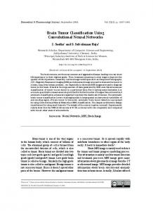
√∑ N ˆ2 ˆ σ ˜ = k=1 (Ik − I) /N , where I denotes the gray-value of the highest frequency. Besides, in order to process the MR images as common images, we also change their intensity range to 0-255 linearly. We take T2 for an example to show the effect of our normalization method. Fig.1 shows 30 T2 MR images’ intensity histograms before and after normalization. The 30 T2 MR images come from BRATS 2013 training dataset. It can be seen from Fig.1 that our normalization method can try to make different MR images have similar intensity distributions, while guarantee their histogram shapes unchanged. In most cases, the gray value of the highest frequency is close to the intensity of white matter. Therefore, transforming the gray value of the highest frequency to the same level is equivalent to transforming the intensity of white matter to the same level. Then, after normalizing the revised deviation, the similar intensities in different MR images can roughly have the similar tissue meaning.
(a)
(b)
Fig. 1. Comparison of 30 T2 intensity histograms before and after intensity normalization. (a). Before normalization(after N4ITK); (b). After normalization
2.2
Brain tumor segmentation model
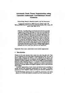
Our brain tumor segmentation model consists of two parts, a Fully Convolutional Neural Network (FCNN) and Conditional Random Field (CRF), as shown in Fig.2. The proposed model was trained by three steps, using image patches and slices respectively. In the testing phase, it can segment brain images slice by slice. Next, we will introduce each part of the proposed segmentation model in detail. FCNN FCNN contains the majority of parameters in our whole segmentation model. It was trained based on image patches, which were extracted from slices of the axial view. Training FCNN by patches can avoid the problem of lacking training samples, as thousands of patches can be extracted from one image. It can also help to avoid the training sample imbalance problem, because the number and position of training samples for each class can be easily controlled by
4
Fig. 2. The structure of our brain tumor segmentation model
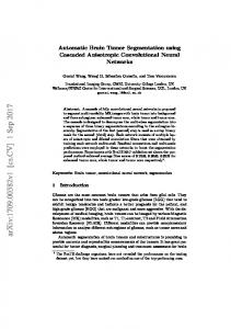
using different patch sampling schemes. In our experiment, we sampled training patches randomly from each training subject and kept the number of training samples for each class equal (5 classes in total, including normal tissue, necrosis, edema, non-enhancing core, and enhancing core). As we didn’t reject patches sampled in the same place, there existed duplicated training samples. Fig.3 shows the structure of the proposed FCNN. Similar to the cascaded architecture proposed in [12], the inputs of our FCNN network also have two different sizes. Passing through a series of convolutional and pooling layers, the large inputs turn into feature maps with the same size of small inputs. These feature maps and small inputs are sent into the following network together. In this way, when we predict the center pixel’s label, the local information and the context information in larger scale can be taken into consideration at the same time. Compared with the cascaded architecture proposed in [12], the two branches in our FCNN was trained simultaneously, while the two branches in the cascaded architecture in [12] was trained in different steps. Besides, our FCNN network has more convolutional layers. FCNN is a fully convolutional neural network and the stride of each layer is set to 1. Therefore, even though it was trained by patches, it can segment brain images slice by slice.
Fig. 3. The structure of our FCNN network
5
CRF Let’s briefly review conditional random field first. Consider an image I composed by a set of pixels {I1 , I2 , . . . , IM }, where M denotes the number of pixels in this image. Each pixel Ii has a label xi , xi ∈ L = {l1 , l2 , . . . , lk }. L is a set of labels, showing the range of value for xi . The energy function of CRF is written as: ∑ ∑ E(x) = Φ(xi ) + Ψ (xi , xj ), i ∈ {1, 2, 3, . . . , M }, j ∈ Ni (1) i
i,j∈Ni
Φ(xi ) is the unary term, representing the cost of assigning label xi to the pixel Ii . Ψ (xi , xj ) is the pairwise term, representing the cost of assigning label xi and xj to Ii and Ij respectively. Ni represents the neighborhood of pixel Ii . Using CRF to segment an image is to find a set of xi to make the energy function have minimum value. In order to improve segmentation accuracy and get a global optimized result, fully connected CRF can be used, which is computing pairwise potentials on all pairs of pixels in the image [17]. The energy function of fully connected CRF is as follows: ∑ ∑ E(x) = Φ(xi ) + Ψ (xi , xj ), i, j ∈ {1, 2, 3, . . . , M } (2) i
i