Hinkkanen, M. & Luomi, J. Title: Braking Scheme for Vector-Controlled Induction Motor Drives. Equipped With Diode Rectifier Without Braking Resistor. Year:.
This is an electronic reprint of the original article. This reprint may differ from the original in pagination and typographic detail.
Author(s):
Hinkkanen, M. & Luomi, J.
Title:
Braking Scheme for Vector-Controlled Induction Motor Drives Equipped With Diode Rectifier Without Braking Resistor
Year:
2006
Version:
Post print
Please cite the original version: Hinkkanen, M. & Luomi, J. 2006. Braking Scheme for Vector-Controlled Induction Motor Drives Equipped With Diode Rectifier Without Braking Resistor. IEEE Transactions on Industry Applications. Volume 42, Issue 5. 1257-1263. ISSN 0093-9994 (printed). DOI: 10.1109/tia.2006.880852. Rights:
© 2006 Institute of Electrical & Electronics Engineers (IEEE). Personal use of this material is permitted. Permission from IEEE must be obtained for all other uses, in any current or future media, including reprinting/republishing this material for advertising or promotional purposes, creating new collective works, for resale or redistribution to servers or lists, or reuse of any copyrighted component of this work in other work.
All material supplied via Aaltodoc is protected by copyright and other intellectual property rights, and duplication or sale of all or part of any of the repository collections is not permitted, except that material may be duplicated by you for your research use or educational purposes in electronic or print form. You must obtain permission for any other use. Electronic or print copies may not be offered, whether for sale or otherwise to anyone who is not an authorised user.
Powered by TCPDF (www.tcpdf.org)
1
Braking Scheme for Vector-Controlled Induction Motor Drives Equipped With Diode Rectifier Without Braking Resistor Marko Hinkkanen, Member, IEEE, and Jorma Luomi, Member, IEEE
Abstract—This paper deals with sensorless vector control of PWM-inverter-fed induction motor drives equipped with a threephase diode rectifier. An electronically controlled braking resistor across the dc link is not used. Instead, the power regenerated during braking is dissipated in the motor while a dc-link overvoltage controller limits the braking torque. Losses in the motor are increased by an optimum flux-braking controller, maximizing either the stator voltage or the stator current depending on the speed. Below the rated speed, the braking times are comparable to those achieved using a braking resistor. The proposed braking scheme is very simple and causes no additional torque ripple. Experimental results obtained using a 2.2-kW induction motor drive show that the proposed scheme works well. Index Terms—DC-link capacitor, field weakening, flux braking, overvoltage.
I. I NTRODUCTION Induction motor drives are usually equipped with a costeffective diode rectifier, allowing the power flow only from the mains to the dc link. An electronically controlled braking resistor across the dc link can be used for dissipating the regenerated braking power, but it increases the price and size of a drive. An inexpensive approach is to dissipate the braking power directly in the motor. Generally, the most effective power dissipation can be achieved in low-power motors due to their large per-unit resistances. In the conventional dc-braking method, a zero-frequency current is fed to the stator winding, resulting in zero air-gap power. DC braking is suitable only for stopping the motor, and its braking torque is small. A higher braking torque can be reached at negative slip values if the power from the stator into the inverter is controlled to zero and the motor losses are sufficient. In a method called flux braking [1], the motor losses are made higher by increasing the flux. The method is suitable for vector control, the braking can be controlled, and the motoring mode can be entered whenever desired. An efficient but complicated braking method is proposed in [2], where a square-wave current is superimposed on the flux-producing current component. Furthermore, a PI-type dclink overvoltage controller—limiting the braking torque based on the measured dc-link voltage—is used, but no details of the controller or its parameter selection are given. In [3], a high-frequency voltage is superimposed on the stator voltage for inducing losses but, unfortunately, large torque pulsations appear in this dual-frequency braking. A high braking torque can be achieved using high-slip braking [4], but the method
idi Rd udi
Ld
id
Cd
ud
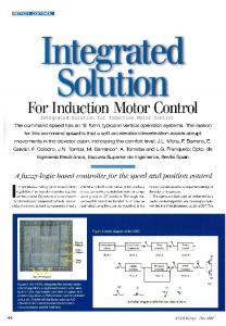
Fig. 1. Simplified model of diode rectifier and dc link.
is not well suited to vector-controlled drives due to the very low flux. This paper proposes a simple P-type dc-link overvoltage controller, which can be easily added to a speed or torque controller. The principle of flux braking is used to increase the losses. Depending on the speed, the proposed flux-braking controller maximizes either the stator voltage or the stator current. The losses are maximized, and the proposed controller can thus be considered as an optimum flux-braking controller. It is integrated with a field-weakening controller, resulting in fast dynamic response and smooth transitions between different operating modes. II. S YSTEM M ODEL A. Diode Rectifier and DC Link The models of the drive system components are presented in the following. A simplified model of the three-phase diode rectifier and the dc link is shown in Fig. 1. The corresponding differential equations are didi = udi − ud − Rd idi , dt dud Cd = idi − id dt Ld
idi ≥ 0
(1a) (1b)
where idi is the current at the output of the rectifier and udi the ideal rectified voltage. The current and the voltage at the input of the inverter are id and ud , respectively. The dclink inductance, capacitance, and resistance are Ld , Cd , and Rd , respectively. The mains inductance can be approximately included in the parameters Ld and Rd [5]. From (1), the rate of change of the energy stored in the capacitor can be expressed as Ld di2di Cd du2d = udi idi − Rd i2di − − pd (2) 2 dt 2 dt where pd = ud id is the power into the inverter.
2
B. Induction Motor and Mechanics The dynamic model corresponding to the inverse-Γ equivalent circuit [6] of the induction motor will be used. In a general reference frame, the voltage equations are us = Rs is +
u′s,ref
dψ s
+ jωk ψ s (3a) dt dψ R + j (ωk − ωm ) ψ R (3b) 0 = RR iR + dt where us is the space vector of the stator voltage, is the space vector of the stator current, Rs the stator resistance, and ωk the electrical angular speed of the reference frame. The rotor resistance is RR , the rotor current iR , and the electrical angular speed of the rotor ωm . The stator and rotor flux linkages are ψ s = (L′s + LM ) is + LM iR ,
ψ R = LM (is + iR )
(6)
where J is the total moment of inertia of the mechanical system, TL the load torque, and b the viscous friction coefficient. The stator power can be expressed as 3 Re{us i∗s } = pCus + pf + pCur + pm (7) 2 where the resistive losses in the stator and rotor are 3 3 (8) pCus = Rs i2s , pCur = RR i2R 2 2 respectively, and the rate of change of the magnetic energy is � � 2 3 L′s di2s 1 dψR (9) pf = + 2 2 dt 2LM dt ps =
The magnitude of the stator current is is = |is | and the magnitudes of other space vectors are defined similarly. The mechanical power is pm = T e
2 3 ψR ωm ωr ωm = p 2 RR
is,ref
ωm,ref
ud
us,ref
Current control
Speed control
ˆ
ejϑs
ˆ
PWM
is
e−jϑs ϑˆs ω ˆm
respectively, where LM is the magnetizing inductance and the stator transient inductance. Iron losses are ignored here, but they will be considered in Section V. The electromagnetic torque is given by n o 3 Te = p Im is ψ ∗R (5) 2 where p is the number of pole pairs and the symbol ∗ marks the complex conjugate. The equation of motion is b J dωm = T e − T L − ωm p dt p
Voltage control
(4) L′s
Stator reference frame
Estimated rotor flux reference frame
Speedadaptive observer
IM
Fig. 2. Simplified block diagram of rotor-flux-oriented control system. Block “Speed control” includes speed controller augmented with proposed dc-link overvoltage controller. Block “Voltage control” includes proposed flux-braking controller integrated with field-weakening controller.
C. Speed-Sensorless Control System In the following sections, a speed-sensorless rotor-fluxoriented control system is assumed. A simplified block diagram of the system is shown in Fig. 2. The stator current is and the dc-link voltage ud are measured. The rotor flux estimate (whose amplitude is denoted by ψˆR and angle by ϑˆs ) and the rotor speed estimate ω ˆ m can be obtained using a speed-adaptive flux observer [7], [8]. The speed controller is augmented with the proposed dclink overvoltage controller as described in Section III. The proposed flux-braking controller is integrated with the fieldweakening controller according to Section IV. This combined field-weakening and flux-braking controller is referred to as voltage controller in Fig. 2.
III. DC-L INK OVERVOLTAGE C ONTROL A. Principle During braking, the dc-link voltage ud rises and the current idi decreases to zero according to (1a). When idi = 0, the power balance (2) reduces to
(10)
where ωr = ωs − ωm is the angular slip frequency and ωs the angular frequency of the rotor flux. The air-gap power pδ = pCur + pm transferred into the rotor can be expressed as �2 � 2 3 1 dψR 3 ψR pδ = ωr ωs (11) + 2 RR dt 2 RR The inverter is modeled by three ideal changeover switches, i.e., ps = pd holds. Steady-state operation without a braking 2 resistor is possible if the condition TL ωm /p+bωm /p2 +pCus + pCur ≥ 0 holds.
Cd du2d = −pd = −pm − pf − pCu 2 dt
(12)
where (7) is also used and the resistive losses are pCu = pCus + pCur . Since the rate of change pf of the magnetic energy is usually small compared with the other terms in (12), pf = 0 will be assumed. A simple proportional controller including the feedforward compensation of pCu can be used to control the square u2d of the dc-link voltage, pm = −
� αu Cd 2 ud,max − u2d − pˆCu 2
(13)
3
where ud,max is the maximum dc-link voltage and pˆCu the estimate of the losses pCu . The feedback (13) in (12) results in the closed-loop system � du2d 2 (pCu − pˆCu ) = αu u2d,max − u2d − dt Cd
(14)
where αu is the bandwidth and pCu − pˆCu acts as a disturbance. According to (14), the dc-link voltage ud in steady state is r 2 (pCu − pˆCu ) (15) ud = u2d,max − Cd αu B. Control Algorithm The estimated rotor flux reference frame is considered. The components of the stator current vector correspond to is = isd + jisq , and the components of other space vectors are defined similarly. Based on (10), the mechanical power pm can be controlled via the electromagnetic torque or the torqueproducing current component isq . The dc-link overvoltage controller can be implemented as a dynamic limit isqu for the reference of the torque-producing current component, � � � 2 αu Cd 2 2 (16) ud,max − ud + pˆCu isqu = 2 3ψˆR ω ˆm
where the resistive losses can be estimated as � 3� pˆCu = (17) Rs (i2sd + i2sq ) + RR i2sq 2 If the measured dc-link voltage is low-pass filtered, the bandwidth αu should be substantially lower than the bandwidth of the filtering. According to (15), the bandwidth αu and the capacitance Cd also affect the steady-state control error in ud during braking. The limits corresponding to the maximum stator current and the breakdown torque are also evaluated. The maximum stator current is,max is taken into account by the limit q (18) isqi = i2s,max − i2sd,ref
where isd,ref is the reference of the flux-producing current component. The breakdown torque is taken into account by the limit isqb = ψˆR /L′s + isd,ref , ideally corresponding to the condition ψsd = ψsq , where ψsd and ψsq are the components of the stator flux in the rotor flux reference frame. The actual limit is the minimum of the preceding limits, ( min {isqb , isqi , isqu } , if i′sq,ref ω ˆm < 0 isq,max = (19) min {isqb , isqi } , if i′sq,ref ω ˆm ≥ 0 i′sq,ref
where is the reference of the torque-producing current component before limitation. The overvoltage limit isqu is taken into account in (19) only if the estimated mechanical power is negative. The output of the speed controller is ( i′ , if |i′sq,ref | ≤ isq,max (20) isq,ref = sq,ref ′ sign(isq,ref )isq,max , if |i′sq,ref | > isq,max Compared with the controller without the dc-link overvoltage controller, only (16) has been added and (19) modified.
IV. F LUX B RAKING
AND
F IELD W EAKENING
In flux braking, the motor losses are made higher by increasing the flux. The flux is limited by the maximum current at low speeds and by the maximum voltage at high speeds. For a high braking torque, the controller should thus maximize either the stator current or the stator voltage depending on the speed. In the following, the flux-braking controller is integrated with the field-weakening controller. A. Preliminaries Conventionally, field weakening is achieved by decreasing the flux reference inversely proportionally to the rotor speed. Alternatively, the flux reference can be determined based on the error between the reference voltage and the maximum available voltage [9]. A simpler method is obtained by excluding the conventional flux controller [10]; the flux-producing current component is controlled and limited according to1 � � disd,ref = γf u2s,max − (u′s,ref )2 , dt
−is,max ≤ isd,ref ≤ isdN (21) where γf is the controller gain, us,max the maximum available stator voltage, u′s,ref the magnitude of the unlimited voltage reference from the current controller, and isdN the rated value of the flux-producing current component. The algorithm (21) is adopted here due to its simplicity and since a flux-braking controller can easily be included in it. The flux dynamics corresponding to the algorithm (21) can be studied using small-signal linearization. The current controller is assumed to be significantly faster than the flux dynamics. Therefore, from the viewpoint of the flux dynamics, the stator voltage components in the rotor flux reference frame are in steady state, i.e. usd = −ωs ψsq = −ωs L′s isq
usq = ωs ψsd = ωs (ψR + L′s isd )
(22a) (22b)
where Rs = 0 is assumed. Furthermore, isd,ref = isd in (21) due to the fast current controller and u′s,ref = us are assumed. The small-signal linearized model of the flux dynamics is obtained using (21) and (22), and by taking the open-loop dynamics of the rotor flux into account. The result is � � 2γf L′s u2sq0 d˜isd ˜isd + 1 ψ˜R (23a) =− dt ψsd0 L′s dψ˜R RR ˜ = RR˜isd − ψR (23b) dt LM where ˜isd and ψ˜R refer to the deviation about the operating point, and the operating-point quantities are marked by the subscript 0. The gain γf = RR ψsd0 /(L′s usq0 )2 results in eigenvalues approximately at (−1 ± j)RR /L′s , whereas a smaller γf reduces the damping. In the √ field-weakening operation, ψsd0 ≈ ψR0 and usq0 ≈ udN / 3, leading to a practical gain selection rule 3RR ψˆR (24) γf = ′ (Ls udN )2 1 Actually,
the limitation 0.1 · isdN ≤ isd,ref ≤ isdN is used in [10].
4
where udN is the nominal average value of the dc-link voltage. The gain (24) equals approximately the gain proposed in [10], but is simpler to implement. According to the eigenvalues, flux dynamics fast enough can be achieved using (21), and a conventional flux controller is not needed. A detailed analysis of the algorithm (21) can be found in [10]. B. Control Algorithm The flux-braking controller is integrated with the fieldweakening controller according to � � γf u2s,max − (u′s,ref )2 , if braking or disd,ref = field weakening (25) dt αb (isdN − isd,ref ) , otherwise u′s,ref
The field weakening is true if > us,max or isd,ref < isdN holds. The braking is true if isq,max = isqu and isq,ref 6= i′sq,ref hold, where the limit isqu is obtained from the dc-link overvoltage controller (16). Since the braking condition may change its value back and forth, a filter having the bandwidth αb is used to decrease isd,ref to its rated value isdN after braking. The reference is limited to −is,max < isd,ref < isd,max , where the maximum value is (q i2s,max − i2squ , if braking (26) isd,max = is,max , otherwise When braking, the limit (26) allows the torque-producing current component to be controlled by the dc-link overvoltage controller, while the remaining part of the maximum current can be used to increase the losses by the flux-producing current component. The gain (24) is also used in the flux-braking mode in order to achieve smooth transitions between the fluxbraking and field-weakening modes. √ When braking, the maximum voltage us,max = ud / 3 corresponding to the linear modulation region is used. Otherwise, the maximum voltage us,max corresponds to the inverter voltage hexagon boundaries. When the voltage reference us,ref is located in the first sector, this boundary can be calculated as ud , 0 ≤ ϑ ≤ π/3 (27) us,max = √ 3 sin(ϑ + π/3) where ϑ is the angle of us,ref in the stator reference frame.
TABLE I D ATA OF 2.2- K W M OTOR D RIVE Rated values of motor Speed Frequency Line-to-line voltage Current Torque TN
1 436 r/min 50 Hz 400 V, rms 5.0 A, rms 14.6 Nm
Motor parameters Stator resistance Rs Rotor resistance RR Stator transient inductance L′s Magnetizing inductance LM Total moment of inertia J Viscous friction coefficient b
3.7 Ω 2.1 Ω 0.021 H 0.224 H 0.0155 kgm2 0.0025 Nm·s
DC link Nominal dc-link voltage udN Inductance Ld Capacitance Cd
540 V 8.1 mH 235 µF
where the rotor flux reference frame is used. The stator iron losses can be approximated as � � ωs2 ψs2 ωs + (1 − kHy ) 2 (29) pFe = kHy 2 pFeN ωsN ωsN ψsN
The iron losses in the rated operating point are pFeN , the rated angular stator frequency is ωsN , and the rated stator flux ψsN . The proportion of the hysteresis losses in the rated operating point is determined by the constant kHy . In steady state, the square of the stator flux in (29) can be expressed as 2
2
ψs2 = [(LM + L′s ) isd ] + (L′s isq )
(30)
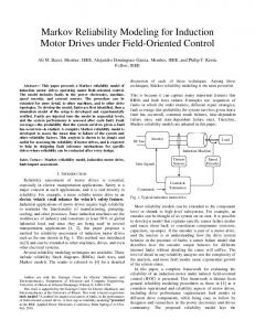
To avoid rising of the dc-link voltage, the stator power ps ≥ 0 should hold. For loss maximization, the magnitude of the stator current should equal its maximum value, i.e., i2sd +i2sq = i2s,max , if possible. The steady-state characteristics of the three braking methods are evaluated assuming the rated stator current and the √ maximum stator voltage us,max = udN / 3. The data of a 2.2kW motor given in Table I are used. The iron losses pFeN = 102 W in the rated operating point and the constant kHy = 0.75. The magnetic saturation is taken into account by using the measured magnetizing inductance LM as a function of isd [11]. The resulting braking torque and the corresponding current components as a function of the rotor speed are shown in Fig. 3.
V. S TEADY-S TATE C HARACTERISTICS In the following, the steady-state characteristics of the proposed braking method are compared with dc braking and high-slip braking. Similar comparisons with dc braking can be found for the braking scheme based on superimposing a square-wave current on the flux-producing current component in [2, Fig. 5] and for the dual-frequency braking method in [3, Fig. 7]. The analysis is based on the motor model of Section II-B augmented with iron losses. It is assumed that the iron losses do not affect the stator current. Consequently, the power (7) in steady state can be expressed as � � 3� Rs i2sd + i2sq + RR i2sq + LM isd isq ωm + pFe (28) ps = 2
A. DC Braking In the dc-braking method, the angular stator frequency is ωs = 0, leading to the air-gap power pδ = 0 in steady state according to (11), and the angular slip frequency is ωr = −ωm . The ratio of the current components in steady state is isq LM = ωr (31) isd RR The dash-dotted curves in Fig. 3 depict the achievable braking torque and the current components as a function of the rotor speed. Since the air-gap power pδ is zero, the stator power is ps = pCus and the mechanical power is pm = pCur ≈ (3/2)RR i2s .
5
Te /TN
0 −0.5
isd (p.u.)
−1 1 0.5
isq (p.u.)
0 0 −0.5 −1 0.2
0.4
0.6 ωm (p.u.)
0.8
1
Fig. 3. Braking torque (first subplot) at rated stator current as function of rotor speed. Corresponding isd and isq are shown in second and third subplot, respectively. Solid line corresponds to proposed method, dashed line to highslip √ braking [4], and dash-dotted line to dc braking. Base values are: current 2·5.0 A and angular frequency 2π·50 rad/s.
Based on Fig. 3, the rotor flux has to be decreased almost to zero. Since the rotor flux cannot be changed instantly, small values of the rotor flux are problematic if the braking is interrupted and a motoring torque is desired. Furthermore, since the slip is usually larger than the breakdown slip, the braking operation may be uncontrollable. B. High-Slip Braking A braking power larger than that of the dc-braking method can be achieved—without increasing the current or the maximum voltage—by controlling the stator power ps to zero. Unlike in the dc-braking method, the stator losses also contribute to the braking power since they are fed by the motor instead of the inverter. Inserting ps = 0 into (28) and using (31), two real-valued solutions of the angular slip frequency ωr can be obtained (except at low speeds when the losses are larger than the mechanical power). Both solutions appear in the regenerating mode, where ωr ωs < 0. The solution giving the larger |ωr | corresponds to the high-slip braking method [4]. The dashed curves in Fig. 3 show the achievable braking torque and the corresponding current components as a function of the rotor speed. The mechanical power during braking is pm ≈ pCus + pCur ≈ (3/2)(Rs + RR )i2s . The braking torque is more than twice that of the dc-braking method. In both methods, the rotor flux is very small, leading to similar problems. C. Proposed Method The proposed method corresponds to the solution of ps = 0 having the smaller |ωr |. The solid curves in Fig. 3 depict the achievable braking torque and the corresponding current components as a function of the rotor speed. It can be seen that the stator current is decreased at speeds larger than 0.83 p.u. due to the stator voltage reaching its maximum value.
The resistive stator losses pCus equal those of the high-slip braking method (at speeds lower than 0.83 p.u. in Fig. 3) while the rotor losses pCur are negligible. However, the iron losses pFe are significant since the current component isd is close to the maximum current. The mechanical power during braking is pm ≈ pCus + pFe ≈ (3/2)Rs i2s + pFe . The braking torque is larger than that of dc braking but smaller than that of high-slip braking. The problems related to the small flux and high slip are avoided: the motoring torque can be rapidly generated and the drive can always be controlled since the slip is smaller than the breakdown slip. It is worth noticing that the proposed dc-link overvoltage controller finds ps = 0 automatically by reducing |ωr | while the proposed flux-braking controller maximizes the stator current or the stator voltage by increasing isd . VI. E XPERIMENTAL S ETUP
AND
PARAMETERS
The operation of the proposed braking scheme was investigated experimentally. A 2.2-kW four-pole induction motor was fed by a frequency converter controlled by a dSPACE DS1103 PPC/DSP board, and a permanent-magnet servo motor was used as a loading machine. The data of the induction motor drive are given in Table I. The total moment of inertia J of the experimental setup is 2.2 times the inertia of the induction motor rotor. √ The base values used are: current 2·5.0 A, flux 1.04 Wb, and angular frequency 2π·50 rad/s. The sampling is synchronized to the modulation, and both the switching frequency and the sampling frequency are 5 kHz. The measured dc-link voltage is filtered using a first-order low-pass filter having the bandwidth of 8 p.u. PI-type synchronous-frame current control having the bandwidth of 6 p.u. is employed [12]. The PI speed controller includes active damping [10], and its bandwidth is 0.15 p.u. The maximum stator current is is,max = 1.5 p.u. The bandwidth of the dc-link overvoltage controller is 0.6 p.u., the maximum dc-link voltage ud,max = 1.15·udN, and the filter bandwidth αb = 0.12 p.u. in (25). VII. E XPERIMENTAL R ESULTS Fig. 4 shows experimental results of an acceleration and a speed reversal. The speed reference is stepped from zero to 1 p.u. at t = 0.25 s and reversed at t = 1.25 s. The rated load torque is applied stepwise at t = 0.5 s and removed at t = 1 s. The removal of the load torque and the speed reversal activate the braking scheme. During the braking operation, the dc-link overvoltage controller drives the power pd to zero while the flux-braking controller increases the losses by maximizing first the stator voltage at higher speeds and then the stator current at lower speeds. It can be seen that the response in the dc-link voltage is smooth. Operation in the field-weakening range is depicted in Fig. 5. The speed reference is stepped from zero to 3 p.u. at t = 0.5 s and back to zero at t = 3 s. Since isd,ref is adjusted based on the available voltage, the current references are realizable in the field-weakening range. As predicted by the linearized model in (23), the response of the rotor flux is fast even though no conventional flux controller is used. It can be seen that the
ωm (p.u.)
1 0
2 0 −2 1.5 1
ud /udN
0.5 1.2 1 0.8
0
0.5
1 t (s)
1.5
2
Fig. 4. Experimental results showing acceleration, load torque step, and speed reversal. First subplot shows measured speed (solid), estimated speed (dotted), and speed reference (dashed). Second subplot shows d and q components of measured stator current (solid) and their references (dashed) in estimated rotor flux reference frame. Third subplot depicts estimated rotor flux magnitude. Last subplot presents filtered dc-link voltage used in controllers.
ψˆR (p.u.)
isd , isq (p.u.)
ωm (p.u.)
4 2
1 0 −1 1 0 −1
0
3
6 t (s)
9
12
Fig. 6. Experimental results showing rated load torque step and its reversal at zero speed reference. First subplot shows measured speed (solid), estimated speed (dotted), and speed reference (dashed). Second subplot shows d and q components of measured stator current (solid) and their references (dashed) in estimated rotor flux reference frame. Last subplot depicts components of estimated rotor flux in stator reference frame.
losses are larger than |pm |. The limit isqu in (16) is large at low speeds, and the torque is thus not limited by the dclink overvoltage controller. Depending on the values of the capacitance Cd , the bandwidth αu , and the maximum dc-link voltage ud,max, the limit isqu may become too small at low speeds unless the feedforward compensation pˆCu is used. The accuracy of pˆCu is not crucial, however.
In the proposed braking scheme, the braking power is effectively dissipated in the motor and, consequently, an electronically controlled braking resistor is avoided. The losses in the motor are increased by an optimum flux-braking controller, maximizing either the stator voltage or the stator current, depending on the speed. Experimental results show that the proposed scheme works well. The dc-link overvoltage controller regulates the dc-link voltage without overshoots. The braking scheme is very simple, allows significant reduction of the braking time below the rated speed, and causes no additional torque ripple.
1 0 −1 1 0.5 0 1.2
ud /udN
0
VIII. C ONCLUSION
0 2
1 0.8
0.1
−0.1
−1
ψˆRα , ψˆRβ (p.u.) isd , isq (p.u.)
ψˆR (p.u.)
isd , isq (p.u.)
ωm (p.u.)
6
0
ACKNOWLEDGMENT 1
2 t (s)
3
4
The authors gratefully acknowledge the financial support given by ABB Oy.
Fig. 5. Experimental results showing operation in field-weakening range. Explanations of curves are as in Fig. 4.
R EFERENCES
dc-link overvoltage controller works well and no overshoots appear in the dc-link voltage. The flux-braking principle is not useful in the field-weakening range. Fig. 6 depicts a load torque step and its reversal at zero speed reference. The rated load torque is stepwise applied at t = 1 s, reversed at t = 5 s, and removed at t = 9 s. The mechanical power pm is negative at transients, but the
[1] P. Tiitinen and M. Surandra, “The next generation motor control method, DTC direct torque control,” in Proc. IEEE PEDES’96, vol. 1, New Delhi, India, Jan. 1996, pp. 37–43. [2] J. Jiang and J. Holtz, “An efficient braking method for controlled ac drives with a diode rectifier front end,” IEEE Trans. Ind. Applicat., vol. 37, no. 5, pp. 1299–1307, Sept./Oct. 2001. [3] M. Rastogi and P. W. Hammond, “Dual-frequency braking in AC drives,” IEEE Trans. Power Electron., vol. 17, no. 6, pp. 1032–1040, Nov. 2002. [4] M. M. Swamy, T. Kume, Y. Yukihira, S. Fujii, and M. Sawamura, “A novel stopping method for induction motors operating from variable frequency drives,” IEEE Trans. Power Electron., vol. 19, no. 4, pp. 1100– 1107, July 2004.
7
[5] P. C. Krause, O. Wasynczuk, and S. D. Sudhoff, Analysis of Electric Machinery and Drive Systems. Piscataway, NJ: IEEE Press, 2002. [6] G. R. Slemon, “Modelling of induction machines for electric drives,” IEEE Trans. Ind. Applicat., vol. 25, no. 6, pp. 1126–1131, Nov./Dec. 1989. [7] M. Hinkkanen, “Analysis and design of full-order flux observers for sensorless induction motors,” IEEE Trans. Ind. Electron., vol. 51, no. 5, pp. 1033–1040, Oct. 2004. [8] M. Hinkkanen and J. Luomi, “Stabilization of regenerating-mode operation in sensorless induction motor drives by full-order flux observer design,” IEEE Trans. Ind. Electron., vol. 51, no. 6, pp. 1318–1328, Dec. 2004. [9] H. Grotstollen and J. Wiesing, “Torque capability and control of a saturated induction motor over a wide range of flux weakening,” IEEE Trans. Ind. Electron., vol. 42, no. 4, pp. 374–381, Aug. 1995. [10] L. Harnefors, K. Pietil¨ainen, and L. Gertmar, “Torque-maximizing fieldweakening control: design, analysis, and parameter selection,” IEEE Trans. Ind. Electron., vol. 48, no. 1, pp. 161–168, Feb. 2001. [11] M. Hinkkanen and J. Luomi, “Parameter sensitivity of full-order flux observers for induction motors,” IEEE Trans. Ind. Applicat., vol. 39, no. 4, pp. 1127–1135, July/Aug. 2003. [12] F. Briz, M. W. Degner, and R. D. Lorenz, “Analysis and design of current regulators using complex vectors,” IEEE Trans. Ind. Applicat., vol. 36, no. 3, pp. 817–825, May/June 2000.
Marko Hinkkanen (M’06) was born in Rautj¨arvi, Finland, in 1975. He received the M.Sc.(Eng.) and D.Sc.(Tech.) degrees from Helsinki University of Technology, Espoo, Finland, in 2000 and 2004, respectively. Since 2000, he has been a Research Scientist with the Power Electronics Laboratory, Helsinki University of Technology. His main research interest is the control of electric drives.
Jorma Luomi (M’92) received the M.Sc.(Eng.) and D.Sc.(Tech.) degrees from Helsinki University of Technology, Espoo, Finland, in 1977 and 1984, respectively. In 1980, he joined Helsinki University of Technology, and from 1991 to 1998, he was a Professor at Chalmers University of Technology. Since 1998, he has been a Professor with the Department of Electrical and Communications Engineering, Helsinki University of Technology. His research interests are in the areas of electric drives, electric machines, and numerical analysis of electromagnetic fields.