The present article uses as a blueprint [CY06], which proves a CLT for DPRE, and ... result, which is a CLT on the event of survival on the entire regular growth ...
Branching Random Walks in Random Environment are Diffusive in the Regular Growth Phase Hadrian Heil, Makoto Nakashima, Nobuo Yoshida Abstract We treat branching random walks in random environment using the frame of Linear Stochastic Evolution. In spatial dimensions three or larger, we establish diffusive behaviour in the entire growth phase. This can be seen through a Central Limit Theorem with respect to the population density as well as through an invariance principle for a path measure we introduce.
1 1.1
Introduction Background
Branching random walks (and their time-continuous counterpart branching Brownian motion) are treated, with the result of a central limit theorem (CLT), by Watanabe in [Wat67] and [Wat68]. Smith and Wilkinson introduce the notion of random (in time) environment to branching processes [SW69], and in 1972, the book by Athreya and Ney [AN72] appears and gives an excellent overview of the knowledge of the time. A closely related model, the directed polymers in random environment (DPRE), is studied since the eighties, when the question of diffusivity is treated by Imbrie and Spencer [IS88] as well as Bolthausen [Bol89]. A review can be found in [CSY04]. It took until the new millenium for the time-space random environment known from DPRE to get applied to branching random walks by Birkner, Geiger and Kersting [BGK05]. A (CLT) in probability is proven in [Yos08a], and immediately improved to an almost sure sense in [Nak10] with the help of Linear Stochastic Evolutions (LSE), which were introduced in [Yos08b] and [Yos10]. Linear stochastic evolutions build a frame to a variety of models, including DPRE. For LSE, the CLT was proved in [Nak09]. Shiozawa treats the time-continuous counterpart, namely branching Brownian motions in random environment [Shi09, Shi]. The present article uses as a blueprint [CY06], which proves a CLT for DPRE, and the larger angle of view allowed by the LSE gives the crucial ingredients to conclude our result, which is a CLT on the event of survival on the entire regular growth phase, but under integrability conditions slightly more restrictive than those from [Nak10]. Compared to the case of DPRE, the necessary notational overhead is unfortunately significantly bigger. Speaking of DPRE, it is possible to extend the results of [CY06] to the case where completely repulsive sites are allowed, using the same conditioning-techniques as here. A complementing article by two of the authors on a localization result for BRWRE in the slow growth phase is available as a preprint [HN].
1.2
Branching random walks in random environment
We denote the natural numbers by
N0 = {0, 1, 2, . . . } and N = {1, 2, . . . }. 1
We consider particles in Zd , each performing a simple random walk and branching into independent copies at each time-step. i) At time n = 0, there is one particle born at the origin x = 0. ii) A particle born at site x ∈ Zd at n ∈ N0 is equipped with k eggs with probability qn,x (k) (k ∈ N0 ) independently from other particles. iii) In the next time step, it takes its k eggs to a uniformly chosen nearest-neighbour site and dies. The eggs then are hatched. The offspring distributions qn,x = (qn,x (k))k∈N0 are assumed to be i.i.d. in time-space (n, x). This model is called Branching Random Walks in Random Environment (BRWRE). Let Nn,y be the number of the particles which occupy the site y ∈ Zd at time n. For the proofs in this article, a modeling down to the level of individual particles is needed. First, we define namespaces Vn , n ∈ N0 for the n-th generation particles and VN0 for the particles of all generations together: V0 = {1} = {(1)}, Vn+1 = Vn × N0 ∗ , for n ≥ 0, [ VN0 = Vn . n∈
N
0
Then, we label all particles as follows: i) At time n = 0, there is just one particle which we call 1 = (1) ∈ V0 . ii) A particle at time n is identified with its genealogical chart y = (1, y1 , . . . , yn ) ∈ Vn . If the particle y gives birth to ky particles at time n, then the children are labeled by (1, y1 , . . . , yn , 1), . . . , (1, y1 , . . . , yn , ky ) ∈ Vn+1 . By using this naming procedure, we define the branching of the particles rigorously. This definition is based on the one in [Yos08a]. Note that the particle with name x can be located at x anywhere in Zd . As both informations genealogy and place are usually necessary together, it is convenient to combine them to x = (x, x); think of x and x written very closely together. • Random environment of offspring distibutions: We fix a product measure Q ∈ P(Ωq , Gq ) which describes the i.i.d. offspring distributions assigned to each time-space location. d Set Ωq = P(N0 )N0 ×Z , where P(N0 ) denotes the set of probability measure on N0 : n o X P(N0 ) = q = (q(k))k∈N0 ∈ [0, 1]N0 : q(k) = 1 . k∈
N
0
Each environment q ∈ Ωq is a function (n, x) 7→ qn,x = (qn,x (k))k∈N0 from N0 × Zd to P(N0 ). We interpret qn,x as the offspring distribution for each particle which occupies the time-space location (n, x). The set P(N0 ) is equipped with the natural Borel σ-field induced by the one of [0, 1]N0 . We denote by Gq the product σ-field on Ωq . • Spatial motion: A particle at time-space location (n, x) jumps to some neighbouring location (n+1, y) before it is replaced by its children there. Therefore, the spatial motion should be described by assigning a destination to each particle at each time-space location d (n, x). We define the measurable space (ΩX , GX ) as the set (Zd )N0 ×Z ×VN0 with the d product σ-field, and ΩX 3 X 7→ Xn,x for each (n, x) ∈ N0 ×(Z ×VN0 ) as the projection. We define PX ∈ P(ΩX , GX ) as the product measure such that, ( 1 if |e| = 1, PX (Xn,x = e) = 2d 0 if |e| = 6 1, 2
Figure 1: One realization of the first steps and branchings �H �O �V
? v6
�O �V
�_ (h
•�
? v6 �H �V
�_ (h
H�
V�
O�
�O
Z
�V
�H
o/ ? v6 (h �_ V�
�_ (h 6v ? /o
H�
o/ / ? v6 (h �_
d
0 �H
O�
z• zzzzzzzz z z z z zzz zzzzzz zzzzzzzz zzzz1 zzzzzzzz z z zzzzz o/ h( o/ zzzzzzzz _� ? v6 z z z z � v V� H � ◦ O� �O � %• •0 ? H� �V • ? z ? z ??? ? �_ (h zz z /o 6v /o ? z ? z ???? zzz z z ? z ? z ? z ??? zzzzz ??? 12 11 13? z z zz ???? z z z ???? zzz z z ???? v6 o/ h( _� zzzz ? z ? z y◦� zz !◦ ? ◦�# �H V� O � � O %• �V H� •y �_ (h 6v ? /o 121122 131 o/ h( o/ _� ? v6 !◦ !◦ ◦ V� �H O� �O H� �V •y ? �_ (h /o 6v /o
�_ (h 6v ? /o
�H
�O
o
o/ ? v6 (h �_
�O
h( _� 6v ?
V�
�V
time
V� O� H�
�_ (h 6v ? /o
O� H�
�
•� ?????? ??????? ?????? ?????? ??
�O
o/ ? v6 (h �_ �V
�H
�_ h( 6v ? o/
H�
V� O�
132 ?????
h( _� 6v ?
H�
V�
O�
????? ?????? ?????? ?????? ◦�' �• %• •0
for e ∈ Zd and (n, x) ∈ N0 × (Zd × VN0 ). Here, we interpret Xn,x as the step at time n + 1 if the particle x is located space location x. d • Offspring realization: We define the measurable space (ΩK , GK ) as the set N0 N0 ×Z ×VN0 with the product σ-field, and ΩK 3 K 7→ Kn,x for each (n, x) ∈ N0 × (Zd × VN0 ) as the q projection. For each fixed q ∈ Ωq , we define PK ∈ P(ΩK , GK ) as the product measure such that q PK (Kn,x = k) = qn,x (k)
for all (n, x) = (n, x, x) ∈ N0 × Zd × VN0 and k ∈ N0 .
We interpret Kn,x as the number of eggs of the particle x if it is located at time-space location (n, x). One could directly speak of its children as well. In Figure 1, the first steps in of such a BRWRE are shown. In this particular example, there are only two types of offspring distibutions, one allowing for one or three eggs, the other one for two or none. The cones in the lower part of the picture get their full meaning in Remark 2.1.2. Putting everything together, we arrive at the • Overall construction: We define (Ω, G) by Ω = ΩX × ΩK × Ωq ,
G = GX ⊗ GK ⊗ Gq ,
and with q ∈ Ωq and P q , P ∈ P(Ω, G) by q
P = PX ⊗
q PK
Z ⊗ δq , 3
P =
Q(dq)P q .
Now that the BRWRE is completely modeled, we can have a look at where the particles are: for (n, y) ∈ N0 × (Zd × VN0 ), we define Nn,y = 1{the particle y is located at time-space location (n,y)} . This enables the • Placement of BRWRE into the framework of Linear Stochastic Evolutions: We set the starting condition N0,y = 1y=(0,1) . Then, defining the matrices (An )n via their entries in the manner indicated below, we can describe Nn,y inductively by X Nn,y = Nn−1,x 1{y−x=Xn−1,x , 1≤y/x≤Kn−1,x } ,
x∈Z
=
d ×V
X
x∈Z
N0
Nn−1,x An,yx
d ×V
N0
= (N0 A1 · · · An )y , where y/x is given for x, y ∈ VN0 as k if x = (1, x1 , . . . , xn ) ∈ Vn , for some n ∈ N0 , y = (1, x1 , . . . , xn , k) ∈ Vn+1 y/x = ∞ otherwise, and where
An,yx := 1{y−x=Xn−1,x ,
1≤y/x≤Kn−1,x } .
One-site- and overall population can be defined respectively as X X Nn,y = Nn,(y,y) , and Nn = Nn,y ,
y ∈Z
y∈VN0
d ×V
N0
for n ∈ N0 , y ∈ Zd . Other quantities needed later are the moments of the local offspring distributions X (p) m(p) = Q[m(p) k p qn,x (k), p ∈ N0 , n,x ] with mn,x = k∈
N
0
m = m(1) , and the normalized one-site and overall populations N n,y = Nn,y /mn and N n = Nn /mn . It is easy to see that the expectation of the matrix entries, which is an important parameter in the setting of LSE, computes as ayx := P [A1,xy ] ( P =
1 2d
q(j)
j≥k
0
with
if |x − y| = 1, y/x = k, k ∈ N0 ∗ , otherwise,
� q(j) := Q q0,0 (j) , j ∈ N0 .
Taking sums, we obtain X
y∈(Z
ayx = m, for
N0 )
d ×V
4
x ∈ (Zd × VN0 ).
1.3
Preliminaries
In this and the following subsection, we gather already known properties of BRWRE. (x,x) First, we introduce the Markov chain (S, PSx ) = ((S, S), P(S,S) ) on Zd × VN0 for x = (x, x) ∈ Zd × VN0 , independent of (An )n≥1 , by
PS Sn+1
PSx (S0 = x) = 1, ( P q(j) j≥k � ayx 2d m = = y| Sn = x = m 0
if |x − y| = 1, and y/x = k ∈ N0 ∗ (1.1) otherwise.
where x, y ∈ Zd ×VN0 . The filtration of this random walk will be called Fn = σ(Fn1 ×Fn2 ), with Fn1 := σ(S1 , . . . , Sn ), Fn2 := σ(S1 , . . . , Sn ), n ∈ N0 , and the corresponding sample space Ω1 × Ω2 . Note that we can regard S and S as independent Markov chains on Zd and VN0 , respectively, with S the simple random walk on Zd . Next, we introduce a process which is essential to the proof of our results: ζ0 = 1 and for n ≥ 1, ζn = ζn (S) =
n m Y Am,SSm−1 m=1
aSSm m−1
.
(1.2)
Lemma 1.3.1. ζn is a martingale with respect to the filtration H0 = σ(S0 ), Hn := σ(Am , Sm ; m ≤ n), n ≥ 1. Moreover, we have that Nn,y = mn PS
(0,1)
[ζn : Sn = y] P -a.s. for n ∈ N0 ,
y ∈ Zd × V N .
The proof of this Lemma can be found in [Nak10]. (0,1) We remark that Nn,y = mn PS [ζn : Sn = y]. From this Lemma follows an important result. The following Lemma shows that a phase transition occurs for the growth rate of the total population. Lemma 1.3.2. N n is a martingale with respect to Gn = σ(Am : m ≤ n). Hence, the limit N ∞ = lim N n , exists P -a.s. n→∞
(1.3)
and P [N ∞ ] = 1 or 0. Moreover, P [N ∞ ] = 1 if and only if the limit (1.3) is convergent in L1 (P ). We refer to the case P [N ∞ ] = 1 as regular growth phase and to the other, P [N ∞ ] = 0 as slow growth phase. The regular growth phase means that the growth rate of the total population is of same order as its expectation mn , while the slow growth phase means that, almost surely, the growth rate of the population is lower than the growth rate of its expectation. One can also introduce the notions of ‘survival’ and ‘extinction’. Definition 1.3.3. The event of survival is the existence of particles at all times: {survival} := {∀ n ∈ N0 , Nn > 0}. The extinction event is the complement of survival.
5
1.4
The result
Definition 1.4.1. An important quantity of the model is the population density, which can be seen as a probability measure with support on Zd , ρn,x = ρn (x) :=
Nn,x 1Nn >0 , n ∈ N0 , x ∈ Zd . Nn
Our main result is the following CLT, proven as Corollary 2.2.4 of the invariance principle Theorem 2.2.2. (2) � Theorem 1.4.2. Assume d ≥ 3 and regular growth, as well as m(3) < ∞ and Q (mn,x )2 < ∞. Then, for all bounded continuous function F ∈ Cb (Rd ), in P ( · |survival)-probability, � x � Z X = F (x)ν(dx), ρn (x)F √ lim n→∞ n Rd d x∈
Z
where Cb (Rd ) stands for the set of bounded continuous functions on Rd , and ν for the Gaussian measure with mean 0 and covariance matrix d1 I. Remark 1.4.3. It is the following equivalence, recently proven as [CY, Proposition 2.2.2], that enables us to speak easily of P ( · |survival)-probability: Lemma 1.4.4. If P (N ∞ > 0) > 0 and m < ∞, then {survival} = {N ∞ > 0}, P -a.s.. [CY] handles also the case of slow growth.
2 2.1
Proofs The path measure
Definition 2.1.1. We set, on F∞ , µn (dS) :=
1 PS (ζn dS)1N ∞ >0 Nn
where ζ is defined in (1.2). Additional notations and definitions comprise the shifted processes: for (m, z) ∈ m,z m,z = (N n,y )y∈Zd ×VN , n ∈ N0 respectively by X y m,z m,z m,z Nn+1, Nn, N0, x Am+n+1,x , and y = 1y=z , y= m,z N0 × Zd × VN , we define Ntm,z = (Nn, y )y∈Zd ×VN and N t
x∈Z ×V z = m−n N m,z . y n,y d
N
m, N n,
Using this, we can, with m ≤ n, express µn on a finite time-horizon as m,
µn (S[0,m] = x[0,m] ) = ζm (x[0,m] )
x
m
N n−m PS (S[0,m] = x[0,m] )1N ∞ >0 ; Nn
in particular, X Nn,x 1N ∞ >0 = µn (S[0,n] = x[0,n] ). Nn x :x =x [0,n]
6
n
(2.1)
Note that for B ∈ F∞ , the limit µ∞ (B) = lim µn (B) n→∞
exists P -a.s. because of the martingale limit theorem for PS (ζn : B), which is indeed a positive martingale with respect to the filtration (Gn )n , as can be easily checked, and for N n , see Lemma 1.3.2. Remark 2.1.2. We can write, for B ∈ Fn1 , 1 X n,xn µ∞ (B × Ω2 ) = PS (ζn : (B × Ω2 ) ∩ {Sn = xn })N ∞ 1N ∞ >0 . N ∞ xn The reader who cares to return to the lower part of Figure 1 will be rewarded with an intuitive picture of how we can let run our BRW up to time n = 3 and plug in there the shifted processes, indicated by the dotted cones. Definition 2.1.3. We define the environmental measure conditional on survival, or equivalently, regular growth, by Pe(·) = P
� P (· ∩ N ∞ > 0) . · N ∞ > 0 = P (N ∞ > 0)
Attention: ‘regular growth’ is not the same thing as the ‘regular growth phase’, but the event defined in Definition 1.3.3. Lemma 2.1.4. Assume regular growth. Then, 1 Peµ∞ (· × Ω2 ) is a probability measure on F∞ ,
(2.2)
1 Peµ∞ (· × Ω2 ) � PS on F∞ ,
(2.3)
and where PS denotes the measure of a simple random walk. In order to prove this Lemma, we need the following observation: 1 are such that limm→∞ PS (Bm × Ω2 ) = 0. Then Lemma 2.1.5. Suppose (Bm )m≥1 ⊂ F∞
0 = lim sup Peµn (Bm × Ω2 ) = lim Peµ∞ (Bm × Ω2 ). m→∞ n
m→∞
Proof. We first prove the first equality. For δ > 0, P (µn (Bm × Ω2 )) ≤ P (µn (Bm × Ω2 ) : N n ≥ δ) + P (1N ∞ >0 : N n ≤ δ). We can estimate � � sup P µn (Bm × Ω2 ) : N n ≥ δ ≤ δ −1 sup P N n µn (Bm × Ω2 ) n
n
� PS (ζn : Bm × Ω2 ) = δ −1 sup P N n 1N ∞ >0 Nn n � −1 ≤ δ sup PS P (ζn ) : Bm × Ω2 �
n
= δ −1 PS (Bm × Ω2 ) −−−−→ 0. m→∞
−1 On the other hand, as N n converges Pe-a.s., their distributions are tight, and
lim sup Pe(N n ≤ δ) = 0.
δ→0 n
The second equality follows directly by an application of dominated convergence. 7
Proof of Lemma 2.1.4. The statement (2.2) is in some sense an affirmation of well-definiteness. The proof consists in verifying that Peµ∞ is finitely additive, that Peµ∞ (Ω1 × Ω2 ) = 1, and that F∞ 3 Bn × Ω2 & ∅ ⇒ Peµ∞ (Bn × Ω2 ) → 0. The first two are quite obvious and the third one is a trivial application of the preceding Lemma 2.1.5, as is the absolute continuity (2.3). In the following Proposition, we introduce the variational norm kν−ν 0 kE := sup{ν(A)− ν (A), A ∈ E}, where ν and ν 0 are probability measures on E. This norm will be applied to µn+m (· × Ω2 ) and µ∞ (· × Ω2 ), which are indeed, Pe-a.s., probability measures on Fr1 because of the finiteness of Fr1 , for all r, m, n ∈ N0 . 0
Proposition 2.1.6. In the regular growth phase, � lim sup Pe kµm+n (· × Ω2 ) − µ∞ (· × Ω2 )kFn1 = 0.
m→∞ n
Proof. From (2.1) and its analogue for µ∞ , for n, m ≥ 0, N ∞ kµm+n (· × Ω2 ) − µ∞ (· × Ω2 )kFn1 n,Sn n � N n,Sn � o N sup PS ζn m 1A − ζn ∞ 1A 1N ∞ >0 = N∞ 1 ⊗F 2 N n+m N∞ A=A1 ×Ω2 ∈Fn n ! n,S n,S n N n N ≤ N ∞ PS ζn m − ∞ 1N ∞ >0 N n+m N∞ −1 n,Sn n,Sn � = 1N ∞ >0 N n+m PS ζn |N ∞ N m − N n+m N ∞ | � � −1 n,Sn n,Sn ≤ 1N ∞ >0 N n+m PS ζn |N ∞ N m − N n+m N m | � n,Sn n,Sn � + |N n+m N m − N n+m N ∞ | ≤
|N ∞ − N n+m | n,Sn � n,Sn n,Sn � + PS ζn |N m − N ∞ | . P S ζn N m N n+m
Note that in the first of the right-hand terms, the denominator is cancelled out with n,Sn � PS ζn N m ; so, as N n converges in L1 (P ), the P -expectation of the first term vanishes as m → ∞, and the second one yields n,Sn n,Sn � P PS ζn |N m − N ∞ | � �� n,Sn n,Sn = P PS ζn P |N m − N ∞ | Gn
� = P PS ζn kN m − N ∞ L1 (P ) = kN m − N ∞ kL1 (P ) −−−−→ 0. m→∞
This proves � sup P N ∞ kµm+n − µ∞ kFn1 −−−−→ 0. m→∞
n
Now, we use the same trick with the Chebychev-inequality that gives us a N ∞ in front of the norm as in Lemma 2.1.4: � � Pe kµm+n − µ∞ kFn1 = Pe kµm+n − µkFn1 (1N ∞ >δ + 1N ∞ ≤δ ) � � ≤ δ −1 Pe N ∞ kµm+n − µ∞ kFn1 + 2Pe N ∞ ≤ δ tends to 0 with δ → 0, m → ∞ if we control δ and m approprietely, independently of n. 8
2.2
The main statements
Definition 2.2.1. For n ≥ 1, the rescaling of the path S is defined by (n)
St
√ = Snt / n,
0 ≤ t ≤ 1,
with (St )t≥0 the linear interpolation of (Sn )n∈N . Furthermore,the d-dimensional Wiener-space will be denoted by (W, F W , P W ), where we equip W = {w ∈ C([0, 1] → Rd ); w(0) = 0} with the topology induced by the usual supremum-norm, and where F W is the Borel-σ-algebra and P W the Wiener measure. Theorem 2.2.2. Assume d ≥ 3 and regular growth, and the technical assumptions (2) � m(3) < ∞, P (m0,0 )2 < ∞. Then, for all F ∈ Cb (W), √ � (n) � lim µn F (S· ) = P W F (·/ d) ,
(2.4)
√ � (n) � lim µ∞ F (S· ) = P W F (·/ d) ,
(2.5)
n→∞
n→∞
in Pe-probability. Remark 2.2.3. This is equivalent to Lp (Pe)-convergence for any finite p. This Theorem admits for the following CLT: Corollary 2.2.4. Under the same assumptions as in the Theorem, for all F ∈ Cb (Rd ), lim
Z � x �N n,x √ F = F (x)dν(x), in Pe-probability. n Nn Rd d
X
n→∞ x∈
Z
where ν designs the Gaussian measure with mean 0 and covariance matrix
2.3
1 d I.
Some easier analogue of the main Theorem
The following Proposition is not needed for the proof of our result. We literally propose it nevertheless to the readers attention because the proof is much easier than the one of Theorem 2.2.2, while the proceeding is the same. Basically, it can be done with the onedimensional tools we have at hand from subsection 2.1 and without the technical hassles in Lemmas 2.4.2, 2.4.4, and 2.4.8. We will try to break it down to small parts as much as we can, and refer to these parts in the proof of Theorem 2.2.2. Proposition 2.3.1. Assume regular growth. Then, √ lim Peµn (S (n) ∈ ·) = P W (w/ d ∈ ·), weakly,
(2.6)
√ lim Peµ∞ (S (n) ∈ ·) = P W (w/ d ∈ ·), weakly.
(2.7)
n→∞
n→∞
The following notation will prove useful. Definition 2.3.2. We define · � F (w) = F (w) − P W F ( √ ) , F ∈ Cb (W) d and
BL(W) = {F : W → R; kF kBL := kF k + kF kL < ∞}
9
the set of bounded Lipschitz-functionals on by
W. The two norms are defined respectively
kF k := sup |F (w)|, w∈W � � F (w) − F (w) e kF kL := sup : w 6= w e∈W . kw − wk e Proof of Proposition 2.3.1. The second statement is easier to prove. We attack it first, and use it later to manage the first one. Two ingredients from outside this article will help us to prove (2.7). First, (2.7) is equivalent to lim Peµ∞ (F (S (m) )) = 0 for all F ∈ BL(W), (2.8) m→∞
e.g., [Dud89, Theorem 11.3.3]. Second, we have the following result for the simple random walk (S, PS ), see [AW00]: If (nk )k≥1 ⊂ Z+ is an increasing sequence such that inf k≥1 nk+1 /nk > 1, then for any F ∈ BL(W), m 1 X F (S (nk ) ) = 0, PS -a.s.. (2.9) lim m→∞ m k=1
One of the key ideas of the proof is that in the last line, due to (2.3), we can replace ‘PS -a.s.’ by ‘Peµ(· × Ω2 )-a.s.’, and the statement still holds. This enables us to prove (2.8) by contradiction. Assume that (2.8) does not hold. Then there is some subsequence aml = Peµ∞ (F (S (ml ) )) > c > 0 (or < c < 0). It has bounded domain, so has a convergent subsequence amlk which can be chosen such that nk := mlk satisfies the above inf k≥1 nk+1 /nk > 1. To this nk , we apply (2.9) and integrate with respect to Peµ∞ . By dominated convergence, we can switch integration and limit and get m � 1 Xe lim P µ∞ F (S (nk ) ) = 0. m→∞ m k=1
But this is a contradition to the assumption that all the Peµ∞ (F (S (nk ) )) = Peµ∞ (F (S (mlk ) )) > c (or < c). So we conclude that (2.8) does hold, indeed. Now, it remains to prove (2.6) with the help of (2.7). We need to show the analogue of (2.8): � (2.10) lim Peµn F (S (n) ) = 0 for all F ∈ BL(W). n→∞
For 0 ≤ k ≤ n, we add some telescopic terms: � � Peµn F (S (n) ) = Peµn F (S (n) ) − F (S (n−k) ) � � + Peµn F (S (n−k) ) − Peµ∞ F (S (n−k) ) � + Peµ∞ F (S (n−k) )
(2.11)
We apply what we just proved, i.e. (2.8), and conclude that the last line vanishes for fixed k and n → ∞. The middle one does the same due to Proposition 2.1.6. As for the first line, we note that F is uniformly continuous and that √ (n) (n−k) sup max St − St = O(k/ n) S∈Ω1 0≤t≤1
Hence, (2.10) holds, so that we conclude (2.6) and thus the Proposition.
10
2.4
The real work
In order to prove the statement of Theorem 2.2.2 ‘in probability’, we take the path via ‘L2 ’. While the proceeding is basically the same as in the last section, the notation becomes much more complicated. As a start, we take a copy of our path S: Definition 2.4.1. Let (e S, PeS ) be an independent copy of (S, PS ) defined on the probability 1 2 e e e e space (Ω = Ω × Ω , F) for i = 1, 2, 3, 4. Similarily, we write ζe = ζ(e S), PSeS , and PS Se for the simultaneous product measures and so on. 1 1 e 2 , the following Lemma 2.4.2. For all B ∈ F∞ ⊗ Fe∞ , with the notation B = B × Ω2 × Ω limit exists P -a.s. in the regular growth phase: ⊗2 µ(2) ∞ (B) = lim µn (B),
(2.12)
n→∞
where we define 1
µ⊗2 n (B) =
2 PSe S Nn
ζn ζen 1B
�
1N ∞ >0 ,
Moreover, we have that for all n ∈ N, P -a.s. on {N ∞ > 0}, � � e µ(2) ek )}nk=1 ∞ (S, S)[0,n] = {(xk , x X n,(xn ,xn ) n,(exn ,exn ) 1 N∞ N∞ · (2.13) = 2 N ∞ xn ,exn ∈VN � � e n ) = (xn , x e [0,n] = {(xk , x en ) . · P e ζn ζen : (S, S) ek )}nk=1 , (Sn , S SS
Proof. Firstly, we prove the existence of the limit. We will examine the following two, complementary processes: � X0 = X1 = 0, Xn = Xn (B) = PSeS ζn ζen 1B∩{Sn−1 6=eSn−1 } � Y0 = PSeS (B), Y1 = PSeS ζ1 ζe1 1B , � Yn = Yn (B) = P e ζn ζen 1 . e B∩{Sn−1 =Sn−1 }
SS
First, we prove that P -a.s., Yn converges to 0, independently of B. A consequence of the construction of the BRWRE is that ζn ζen 1{Sn−1 6=eSn−1 ,Sn =eSn } = 0, P ⊗ PSeS -a.s., so that we have � � 0 ≤ P Yn ≤ P PSeS ζn ζen 1Sn−1 =eSn−1 � = P PSeS ζn ζen 1S[0,n−1] =eS[0,n−1] = P PSeS
n−1 Y
(Ak,SSkk−1 )2
k=1
(aSSkk−1 )2 · PSeS
= PSeS
� n−1 Y k=1
=
1 aSSkk−1
1S[0,n−1] =eS[0,n−1]
� P (An,SSnn−1 A
: S[0,n−1]
! e Sn � |Gn−1 ) n,e Sn−1 e Fn−1 , Fn−1 e aSSnn−1 aeSn Sn−1
=e S[0,n−1]
m(2) 1 m2 mn−1 11
� X P A x A y ) ay 1,(0,1) 1,(0,1) x ayx m2 x, y
(2.14)
We made use of the fact that in the third line, because the Ak,SSkk−1 ’s are indicators, we can erase the square. Also erasable is the condition in the P -expectation in the fourth line. After that, the outmost P -expectation can be taken into the first fraction, cancelling out one of the aSSkk−1 ’s. To what remains, the definition of the expectation, using (1.1). This technique is hinted in the second part of the fifth line, and applied similarly to the first part. It follows from the Borel-Cantelli lemma that P -a.s., Yn converges to 0, independently of B. Next, we will check that Xn is a submartingale with respect to Gn . � ) Gn−1 P (Xn |Gn−1 ) = P P e(ζn ζen 1 e B∩{Sn−1 6=Sn−1 }
SS
� = PSeS
ζn−1 ζen−1 1B∩{Sn−1 6=eSn−1 } P
Sn n,Sn−1 aSSnn−1
�A
e Sn n,e Sn−1 e Sn ae Sn−1
A
��
We do not use the following definition again, but we should like to point out its similarity to W to be defined later. The inner P -expectation computes as w(x, x e , y, y e ) :=
=
P [A1,xy A1,exye ]
ayx ayxee 0 1 P [Pi≥k q0,0 (i) Pj≥l q0,0 (j)] P
q(i)
P
q(j)
j≥l i≥k 0 � P �−1 1 j≥min{k,l} q(j)
2d
if ayx ayxee = 0, if x = 6 x e, ayx ayxee 6= 0 e, x=x e, x 6= x y ye 6 0. if y/x = k, y e /e x = l, ax axe = if x = x e , y 6= ye, ayx ayxee 6= 0 x = xe , y = ye, y ye 6 0 if y/x = k, y e /e x = l, ax axe =
e n−1 }, w(Sn−1 , e Using this, we note that, under the condition {Sn−1 = 6 S Sn−1 , Sn , e Sn ) e e e depends only on Sn−1 − Sn−1 , Sn /Sn−1 and Sn /Sn−1 . Thus, we pursue � = PSeS ζn−1 ζen−1 1B∩{Sn−1 6=eSn−1 } (1Sn−1 6=Sen−1 + α1Sn−1 =Sen−1 ) , (2.15) where α = P (m20,0 )/m2 > 1, which is obtained by introducing a PSeS ( · |Fn−1 , Fen−1 )contitional expectation, and remarking that the event B depends only on the random walk-part and the corresponding above fraction only on the children-part, and are thus independent. The calculus reads as follows: � PSeS ζn−1 ζen−1 1{Sn−1 =Sen−1 ,Sn−1 6=Sen−1 } P P � P [ i≥S /S �� q (i) j≥Sen /Sen−1 q0,0 (j)] n n−1 0,0 P P : B Fn−1 , Fen−1 PSeS e n /S e n−1 q(j) i≥Sn /Sn−1 q(i) j≥S � = PSeS ζn−1 ζen−1 1{Sn−1 =Sen−1 ,Sn−1 6=Sen−1 } P P � X P [ i≥x/Sn−1 q0,0 (i) j≥y/Sen−1 q0,0 (j)] en−1 ) P (B|F , F n−1 e S S m2 x,y = PSeS PSeS (ζn−1 ζen−1 1{Sn−1 =Sen−1 ,Sn−1 6=Sen−1 ,B}
� P (m20,0 ) |Fn−1 , Fen−1 ) 2 m
The BRWRE has, due to the strict construction of the ancestry, the feature that ζn−1 ζen−1 1B∩{Sn−1 6=eSn−1 } ≥ ζn−1 ζen−1 1 . So, we continue (2.15) and finish the proof of the submartine B∩{Sn−2 6=Sn−2 }
gale property by � � ≥ PSeS ζn−1 ζen−1 1B∩{Sn−2 6=eSn−2 } = Xn−1 . 12
Notation 2.4.3. For some sequence (an )n≥0 , we set ∆an := an − an−1 for n ≥ 1. This definition is convenient when we treat the Doob-decomposition of the process Xn , i.e. Xn = Mn + An , (2.16) with Mn a martingale, M0 = A0 = 0, and An the increasing process defined by its increments ∆An . The next Lemma deals with the two processes An and Mn : Lemma 2.4.4. A∞ < ∞ and hM i∞ < ∞,
P -a.s..
If we define the process Xn , with B replaced by some Bm , as Xnm = Mnm + Am n , where ) & 0 with m → ∞, we have P ⊗2 (B m e SS
Am −−−→ 0 and hM m i∞ −−−−→ 0, ∞ − m→∞
P -a.s..
m→∞
(2.17)
The proof is postponed a little bit. Applying the ‘B’-version of this Lemma, we get that Xn converges, and by the con−2 −2 e vergence of N n , µ⊗2 n = N n (Xn + Yn )1N ∞ >0 as well, P -a.s. On the event of extinction, the statement is trivial, and we conclude (2.12). The second statement (2.13) follows immediately from the definition. In order to prove Lemma 2.4.4, we also need the so called replica overlap, which is the probability of two particles to meet at the same place: Rn :=
X � Nn,x � Nn
x
1Nn >0 .
This replica overlap can be related to the event of survival via a Corollary of the following general result for martingales [Yos10, Proposition 2.1.2]. Proposition 2.4.5. Let (Yn )n∈N0 be a mean-zero martingale on a probability space with measure E and filtration (Hn )n∈N0 such that −1 ≤ ∆Yn := Yn − Yn−1 , E-a.s. and Xn :=
n Y
(1 + ∆Ym ).
m=1
Then, {X∞ > 0} ⊇ {Xn > 0 for all n ≥ 0} ∩
�X ∞
�
E (∆Yn )2 Hn−1 < ∞ , E-a.s., (2.18) �
�
N =1
� � holds if Yn is square-integrable and E (∆Yn )2 Hn−1 is uniformly bounded. The opposite inclusion is provided by Yn being cube-integrable and � � � � E (∆Yn )3 Hn−1 ≤ const · E (∆Yn )2 Hn−1 . Corollary 2.4.6. Suppose P (N ∞ > 0) > 0 and m(3) < ∞. Then nX o {N ∞ > 0} = {survival} ∩ Rn < ∞ , P -a.s.. n≥0
13
Proof of Lemma 2.4.4. We make a slight abuse in notation writing B(m) and so on as templates for both the cases B and Bm . We can make use of (2.15) and, splitting two times 1 into complementary indicators, get � ∆A(m) = P ∆Xn(m) Gn−1 n � = PSeS ζn−1 ζen−1 1B (m) h � 1Sn−1 6=Sen−1 + α1Sn−1 =Sen−1 1Sn−1 6=eSn−1 1Sn−2 6=eSn−2 � + 1Sn−1 6=Sen−1 + α1Sn−1 =Sen−1 1Sn−1 6=eSn−1 1Sn−2 =eSn−2 i� � − 1Sn−1 6=Sen−1 + 1Sn−1 =Sen−1 1Sn−2 6=eSn−2 .
1Sn−1 6=eSn−1 is implied by the following indicator, while in the second term, 1Sn−1 6=Sen−1 is 0 due to the fact that ζn−1 ζen−1 1Sn−1 6=Sen−1 1Sn−2 =eSn−2 = 0, P ⊗ PSeS In the last term,
a.s. Thus, we can continue � � = PSeS ζn−1 ζen−1 1B (m) (α − 1)1Sn−1 =Sen−1 1Sn−2 6=eSn−2 + α1Sn−1 =Sen−1 1Sn−1 6=eSn−1 1Sn−2 =eSn−2 � � ≤ αPSeS ζn−1 ζen−1 1Sn−1 =Sen−1 1B (m) , The sum ZA =
X
� �
ζn−1 ζen−1 1Sn−1 =Sen−1
n
is PSeS -integrable, thanks to Corollary 2.4.6 together with Lemma 1.3.1 and Lemma 1.3.2. So, summation over all n ∈ N yields ( 0 n � � � � ≤ P hM (m) i∞ > `, N ∞ > 0 + P sup Mn(m) ≥ ε, τ` = ∞ . n
Clearly, the first term on the right-hand-side vanishes as m % ∞, because of (2.17), and so does the second term as can be seen from the following application of Doob’s inequality (for instance [Dur91, p.248]): � � � � (m) P sup Mn(m) ≥ ε, τ` = ∞ ≤ P sup Mn∧τ` ≥ ε n n � � � � −2 (m) −2 ≤ 4ε P hM iτ` ≤ 4ε P hM (m) i∞ ∧ ` . Since ` is arbitrary, (2.25) follows and hence we conclude (2.24).
18
Proof of Theorem 2.2.2. We are going to make use of the experience gathered in proving Proposition 2.3.1. In a very similar manner to the proof of (2.7), for (2.5), we need to show an analogue of (2.8) with the help of an analogue of (2.9). To be more concrete, we show �� ��2 � = 0, (2.26) lim Pe µ∞ F (S (n) ) n→∞
which implies � Pe |µ∞ (F (S (n) ))| −−−−→ 0,
(2.27)
n→∞
and hence the convergence in probability. Indeed, using the same replacement argument, but with (2.23) instead of (2.3), we get � � √ √ �� �� (n) e(n) = (P W )⊗2 G · / d, e·/ d ,S lim Peµ(2) ∞ G S n→∞
for any G ∈ Cb (W × W). In particular, we can take G(w, w) e = F (w)F (w), e and get (2.26), and hence (2.5). The proof of (2.4) works with the same telescopic technique seen in (2.11) used in the proof of (2.6): � � Pe |µn (F (S (n) ))| = Pe |µn (F (S (n) − F (S (n−k) )) � + Pe |µn (F (S (n−k) )) − µ∞ (F (S (n−k) ))| � + Pe |µ∞ (F (S (n−k) ))| Note that the L2 -techniques in this paragraph that lead to (2.27) are needed only for the treatment of the last line; the other two can be dealt with with the same arguments than after (2.11). We still need to prove Corollary 2.4.6. We start with some notation. Notation 2.4.9. Un+1,x :=
Nn,x 1Nn >0 X
mNn
ν Kn,x ≥ 0,
ν=1
Un+1 :=
X x∈
Z
Un+1,x =
d
Nn+1 N 1N >0 = n+1 1N n >0 . mNn n Nn
The (Un+1,x )x∈Zd are independent under P (·|Gn ). It is not difficult to see that, on the event {Nn > 0}, P (Un+1,x |Gn ) = ρn (x), and hence P (Un+1 |Gn ) = 1. Also, with e ci = αρ(x)2 =
m(i) mi ,
1 m2 Nn2
i = 2, 3,
� � 2 2 Gn Nn,x Q m2n,x ≤ P Un+1,x =
n,x 2 � NX �2 � Nn,x m(2) 1 ν P K ≤ =e c2 ρn (x)2 , G n n,x 2N 2 m2 Nn2 m n ν=1
� m(3) 3 Gn ≤ P Un+1,x ρn (x)3 = e c3 ρn (x)3 , again on the event {Nn > 0}. m3 Proof of Corollary 2.4.6. We need to verify the prerequisites of Proposition 2.4.5 which we apply to Xn := N n and ∆Yn :=
X Nn 1N n >0 − 1N n >0 = [Un,x − ρn,x ] ≥ 1. N n−1 x 19
The second moments compute as X � � P (∆Yn )2 Gn = P ( Un,x − ρn−1,x )2 Gn x
=
X
=
X
� X � P (Un,x − ρn−1,x )(Un,y − ρn−1,y ) Gn−1 = P (Un,x − ρn−1,x )2 Gn−1
x,y
x
P
2 Gn−1 Un,x
�
−
ρ2n−1,x
x
Using the observations after Notation 2.4.9, we hence get � Q(m2 ) �X �X � �2 � � m(2) n,x 2 − 1 − 1 ρ ≤ P ≤ ρ2n−1,x ∆Y G n n n−1,x 2 m2 m x x Similar observations lead to estimate for the third moment: � X � � �3 P (∆Yn )3 Gn−1 = P Un,x − ρn−1,x Gn−1 x
� X � = P (Un,x − ρn−1,x )3 Gn−1 x
≤3
� � m(3) �X X � 3 P Un,x + ρ3n−1,x Gn−1 ≤ − 1 ρ3n−1,x . 3 m x x
This proves that all hypotheses of Proposition 2.4.5 are fulfilled and in fact equality holds for (2.18).
References [AN72]
K.B. Athreya and P.E. Ney. Branching processes. Die Grundlehren der mathematischen Wissenschaften. Band 196. Berlin-Heidelberg-New York: SpringerVerlag. XI., 1972.
[AW00]
Mohamed Atlagh and Michel Weber. The almost sure central limit theorem. (Le th´eor`eme central limite presque sˆ ur.). Expo. Math., 18(2):97–126, 2000.
[BGK05] Matthias Birkner, Jochen Geiger, and G¨otz Kersting. Branching processes in random environment – a view on critical and subcritical cases. In Interacting stochastic systems, pages 269–291. Springer, Berlin, 2005. [Bol89]
Erwin Bolthausen. A note on the diffusion of directed polymers in a random environment. Commun. Math. Phys., 123(4):529–534, 1989.
[CSY04] Francis Comets, Tokuzo Shiga, and Nobuo Yoshida. Probabilistic analysis of directed polymers in a random environment: a review. Funaki, Tadahisa (ed.) et al., Stochastic analysis on large scale interacting systems. Papers from the 11th international conference, Hayama, Japan, July 17–26, 2002 and the international conference on stochastic analysis and statistical mechanics, Kyoto, Japan, July 29–30, 2002. Tokyo: Mathematical Society of Japan. Advanced Studies in Pure Mathematics 39, 115-142, 2004. [CY]
Francis Comets and Nobuo Yoshida. Branching Random Walks in Space-Time Random Environment: Survival Probability, Global and Local Growth Rates. Preprint.
20
[CY06]
Francis Comets and Nobuo Yoshida. Directed polymers in random environment are diffusive at weak disorder. Ann. Probab., 34(5):1746–1770, 2006.
[Dud89] Richard M. Dudley. Real analysis and probability. Wadsworth & Brooks/Cole Mathematics Series. Pacific Grove, CA: Wadsworth & Brooks/Cole Advanced Books & Software. xi, 436 p., 1989. [Dur91]
Richard Durrett. Probability. Theory and examples. Wadsworth & Brooks/Cole Advanced Books & Software, Pacific Grove, CA, 1991.
[HN]
Hadrian Heil and Makoto Nakashima. A Remark on Localization for Branching Random Walks in Random Environment. Preprint.
[IS88]
J. Z. Imbrie and T. Spencer. Diffusion of directed polymers in a random environment. J. Stat. Phys., 52(3-4):609–626, 1988.
[Nak09] Makoto Nakashima. Central limit theorem for linear stochastic evolutions. J. Math. Kyoto Univ., 49(1):201–224, 2009. [Nak10] Makoto Nakashima. Almost Sure Central Limit theorem for Branching Random Walks in Random Environment. Ann. Appl. Probab., to appear, 2010. [Shi]
Yuichi Shiozawa. Localization for branching Brownian motions in random environment. To appear in Tohoku Math. J.
[Shi09]
Yuichi Shiozawa. Central Limit Theorem for Branching Brownian motions in Random Environment. J. Stat. Phys., 136:145–163, 2009.
[SW69]
W.L. Smith and W.E. Wilkinson. On branching processes in random environments. Ann. Math. Stat., 40:814–827, 1969.
[Wat67] Shinzo Watanabe. Limit theorem for a class of branching processes. Markov Processes potential Theory. Proc. Sympos. Univ. Wisconsin, Madison 1967, 205-232 (1967)., 1967. [Wat68] Shinzo Watanabe. A limit theorem of branching processes and continuous state branching processes. J. Math. Kyoto Univ., 8:141–167, 1968. [Yos08a] Nobuo Yoshida. Central limit theorem for branching random walks in random environment. Ann. Appl. Probab., 18(4):1619–1635, 2008. [Yos08b] Nobuo Yoshida. Phase transitions for the growth rate of linear stochastic evolutions. J. Stat. Phys., 133(6):1033–1058, 2008. [Yos10]
Nobuo Yoshida. Localization for Linear Stochastic Evolutions. J. Stat. Phys., 138(4/5):960–977, 2010.
21