Dec 5, 2011 - â School of Mathematics, University of Minnesota, 206 Church St. SE, Minneapolis, MN 55455, USA and Faculty of ..... sk,n(x) with fluctuation less than or equal to fk,n at level k ⤠n. ...... [24] James Nolen and Lenya Ryzhik.
Branching Random Walks in Time Inhomogeneous Environments arXiv:1112.1113v1 [math.PR] 5 Dec 2011
Ming Fang∗
Ofer Zeitouni†
November 18, 2011
Abstract We study the maximal displacement of branching random walks in a class of time inhomogeneous environments. Specifically, binary branching random walks with Gaussian increments will be considered, where the variances of the increments change over time macroscopically. We find the asymptotics of the maximum up to an OP (1) (stochastically bounded) error, and focus on the following phenomena: the profile of the variance matters, both to the leading (velocity) term and to the logarithmic correction term, and the latter exhibits a phase transition.
1
Introduction
Branching random walks and their maxima have been studied mostly in space-time homogeneous environments (deterministic or random). For work on the deterministic homogeneous case of relevance to our study we refer to [4] and the recent [1] and [2]. For the random environment case, a sample of relevant papers is [12, 14, 17, 18, 21, 22, 23]. As is well documented in these references, under reasonable hypotheses, in the homogeneous case the maximum grows linearly, with a logarithmic correction, and is tight around its median. Branching random walks are also studied under some space inhomogeneous environments. A sample of those papers are [3, 7, 9, 13, 15, 16, 19]. Recently, Bramson and Zeitouni [5] and Fang [10] showed that the maxima of branching random walks, recentered around their median, are still tight in time inhomogeneous environments satisfying certain uniform regularity assumptions, in particular, the laws of the increments can vary with respect to time and the walks may have some local dependence. A natural question is to ask, in that situation, what is the asymptotic behavior of the maxima. Similar questions were discussed in the context of branching Brownian motion using ∗
School of Mathematics, University of Minnesota, 206 Church St. SE, Minneapolis, MN 55455, USA. The work of this author was partially supported by NSF grant DMS-0804133 † School of Mathematics, University of Minnesota, 206 Church St. SE, Minneapolis, MN 55455, USA and Faculty of Mathematics, Weizmann Institute, POB 26, Rehovot 76100, Israel. The work of this author was partially supported by NSF grant DMS-0804133, a grant from the Israel science foundation, and the Taubman professorial chair at the Weizmann Institute.
1
PDE techniques, see e.g. Nolen and Ryzhik [24], using the fact that the distributions of the maxima satisfy the KPP equation whose solution exhibits a traveling wave phenomenon. In all these models, while the linear traveling speed of the maxima is a relatively easy consequence of the large deviation principle, the evaluation of the second order correction term, like the ones in Bramson [4] and Addario-Berry and Reed [1], is more involved and requires a detailed analysis of the walks; to our knowledge, it has so far only been performed in the time homogeneous case. Our goal is to start exploring the time inhomogeneous setup. As we will detail below, the situation, even in the simplest setting, is complex and, for example, the order in which inhomogeneity presents itself matters, both in the leading term and in the correction term. In this paper, in order to best describe the phenomenon discussed above, we focus on the simplest case of binary branching random walks where the diffusivity of the particles takes two distinct values as a function of time. We now describe the setup in detail. For σ > 0, let N (0, σ 2 ) denote the normal distributions with mean zero and variance σ 2 . Let n be an integer, and let σ12 , σ22 > 0 be given. We start the system with one particle at location 0 at time 0. Suppose that v is a particle at location Sv at time k. Then v dies at time k + 1 and gives birth to two particles v1 and v2, and each of the two offspring ({vi, i = 1, 2}) moves independently to a new location Svi with the increment Svi − Sv independent of Sv and distributed as N (0, σ12 ) if k < n/2 and as N (0, σ22 ) if n/2 ≤ k < n. Let Dn denote the collection of all particles at time n. For a particle v ∈ Dn and i < n, we let v i denote the ith level ancestor of v, that is the unique element of Di on the geodesic connecting v and the root. We study the maximal displacement Mn = maxv∈Dn Sv at time n, for n large. 1 It will be clear that the analysis extends to a wide class of inhomogeneities with finitely many values and ‘macroscopic’ change (similar to the description in the previous paragraph), and to the Galton-Watson setup. A universal result that will allow for continuous change of the variances is more complicated, is expected to present different correction terms, and is the subject of further study. In order to describe the results in a concise way, we recall the notation OP (1) for stochastically boundedness. That is, if a sequence of random variables Rn satisfies Rn = OP (1), then, for any � > 0, there exists an M such that P (|Rn | > M ) < � for all n. An interesting feature of Mn is that the asymptotic behavior depends on the order relation between σ12 and σ22 . That is, while � �p σ 2 log 2 σeff n − β √ eff log n + OP (1) (1) Mn = 2 log 2 is true for some choice of σeff and β, σeff and β take different expressions for different ordering of σ1 and σ2 . Note that (1) is equivalent to say that the sequence {Mn − M ed(Mn )}n is tight and �p � σ M ed(Mn ) = 2 log 2 σeff n − β √ eff log n + O(1), 2 log 2 1
Since one can understand a branching random walk as a ‘competition’ between branching and random walk, one may get similar results by fixing the variance and changing the branching rate with respect to time.
2
where M ed(X) = sup{x : P (X ≤ x) ≤ 12 } is the median of the random variable X. In the following, we will use superscripts to distinguish different cases, see (2), (3) and (4) below. A special and well-known case is when σ1 = σ2 = σ, i.e., all the increments are i.i.d.. In that case, the maximal displacement is described as follows: � �p σ 3 = log n + OP (1); (2) 2 log 2 σ n − √ Mn = 2 2 log 2 the proof can be found in [1], and its analog for branching Brownian motion can be found in [4] using probabilistic techniques and [20] using PDE techniques. This homogeneous case corresponds to (1) with σeff = σ and β = 23 . In this paper, we deal with the extension to the inhomogeneous case. The main results are the following two theorems. Theorem 1. When σ12 < σ22 (increasing variances), the maximal displacement is p �q � σ 2 + σ22 ↑ 2 2 Mn = (σ1 + σ2 ) log 2 n − √1 log n + OP (1), 4 log 2 q σ12 +σ22 and β = 12 . which is of the form (1) with σeff = 2 Theorem 2. When σ12 > σ22 (decreasing variances), the maximal displacement is √ 3(σ1 + σ2 ) 2 log 2(σ1 + σ2 ) ↓ Mn = n− √ log n + OP (1), 2 2 2 log 2 which is of the form (1) with σeff =
σ1 +σ2 2
(3)
(4)
and β = 3.
For comparison purpose, it is useful to introduce the model of 2n independent (inhomogeneous) random walks with centered independent Gaussian variables, with variance profile as above. Denote by Mnind the maximal displacement at time n in this model. Because of the complete independence, it can be easily shown that p � �q σ 2 + σ22 ind 2 2 (σ1 + σ2 ) log 2 n − √1 Mn = log n + OP (1) (5) 4 log 2 p for all choices of σ12 and σ22 . Thus, in this case, σeff = (σ12 + σ22 )/2 and β = 1/2. Thus, the difference between Mn= and Mnind when σ12 = σ22 lies in the logarithmic correction. As commented (for branching Brownian motion) in [4], the different correction is due to the intrinsic dependence between particles coming from the branching structure in branching random walks. Another related quantity is the sub-maximum obtained by a greedy algorithm, which only considers the maximum over all decendents of the maximal particle at time n/2. Applying (2), we find that the output of such algorithm is � � � � p p n 3 σ1 n n 3 σ2 n 2 log 2σ1 − √ + 2 log 2σ2 − √ + OP (1) log log 2 2 2 log 2 2 2 2 2 log 2 2 √ 3(σ1 + σ2 ) 2 log 2(σ1 + σ2 ) = n− √ log n + OP (1). (6) 2 2 2 log 2 3
Comparing (6) with the theorems, we see that this algorithm yields the maximum up to an OP (1) error in the case of decreasing variances (compare with (4)) but not in the case of increasing variances (compare with (3)) or of homogeneous increments (compare with (2)). A few comparisons are now in order. 1. When the variances are increasing, Mn↑ is asymptotically (up to OP (1) error) the same as Mnind , which is exactly the same as the maximum of independent homogeneous random σ 2 +σ 2 walks with effective variance 1 2 2 . 2. When the variances are decreasing, Mn↓ shares the same asymptotic behavior with the sub-maximum (6). In this case, a greedy strategy yields the approximate maximum. 3. With the same set of diffusivity constants {σ12 , σ22 } but different order, Mn↑ is greater than Mn↓ . 4. While the leading order terms in (2), (3) and (4) are continuous in σ1 and σ2 (they coincide upon setting σ1 = σ2 ), the logarithmic corrections exhibit a phase transition phenomenon (they are not the same when we let σ1 = σ2 ). We will prove Theorem 1 in Section 2 and Theorem 2 in Section 3. Before proving the theorems, we state a tightness result. Lemma 1. The sequences {Mn↑ − Med(Mn↑ )}n and {Mn↓ − Med(Mn↓ )}n are tight. This lemma follows from Bramson and Zeitouni [5] or Fang [10]. One can write down a similar recursion for the distribution of Mn to the one in those two papers, except for different subscripts and superscripts. Since the argument there depends only on one step of the recursion, it applies here directly without any change and leads to the tightness result in the lemma. A note on notation: throughout, we use C to denote a generic positive constant, possibly depending on σ1 and σ2 , that may change from line to line.
2
Increasing Variances: σ12 < σ22
In this section, we prove Theorem 1. We begin in Subsection 2.1 with a result on the fluctuation of an inhomogeneous random walk. In the short Subsection 2.2 we provide largedeviations based heuristics for our results. While it is not used in the actual proof, it explains the leading term of the maximal displacement and gives hints about the derivation of the logarithmic correction term. The actual proof of Theorem 1 is provided in subsection 2.3.
2.1
Fluctuation of an Inhomogeneous Random Walk
Let Sn =
n/2 X
Xi +
i=1
n X i=n/2+1
4
Yi
(7)
be an inhomogeneous random walk, where Xi ∼ N (0, σ12 ), Yi ∼ N (0, σ22 ), and Xi and Yi are independent. Define σ12 k n 0≤k≤ , (σ 2 + σ 2 ) n x, 2 2 2 1 sk,n (x) = (8) σ12 n2 + σ22 (k − n2 ) n x, ≤ k ≤ n, (σ12 + σ22 ) n2 2 and
( fk,n =
cf k 2/3 ,
k ≤ n/2,
cf (n − k)
2/3
,
(9)
n/2 < k ≤ n.
As the following lemma says, conditioned on {Sn = x}, the path of the walk Sn follows sk,n (x) with fluctuation less than or equal to fk,n at level k ≤ n. Lemma 2. There exists a constant C > 0 (independent of n) such that P (Sn (k) ∈ [sk,n (Sn ) − fk,n , sk,n (Sn ) + fk,n ] for all 0 ≤ k ≤ n|Sn ) ≥ C, where Sn (k) is the sum of the first k summands of Sn , i.e., k X Xk , k ≤ n/2, k=1 Sn (k) = n/2 k X X Xk + Yk , n/2 < k ≤ n. k=1
k=n/2+1
Proof. Let S˜k,n = Sn (k) − sk,n (Sn ). Then, similar to Brownian bridge, one can check that S˜k,n are independent of Sn . To see this, first note that the covariance between S˜k,n and Sn is Cov(S˜k,n , Sn ) = E S˜k,n Sn − E S˜k,n ESn = E S˜k,n Sn , since ESn = 0 and E S˜k,n = 0. For k ≤ n/2, S˜k,n =
� 1−
σ12 k (σ12 + σ22 ) n2
�X k i=1
n/2 X σ12 k σ12 k X − Xi − 2 i (σ1 + σ22 ) n2 i=k+1 (σ12 + σ22 ) n2
n X
Yi .
i=n/2+1
Expand S˜k,n Sn , take expectation, and then all terms vanish except for those containing Xi2 and Yi2 . Taking into account that EXi2 = σ12 and EYi2 = σ22 , one has Cov(S˜k,n , Sn ) = E S˜k,n Sn �X � n/2 k n X X σ12 k σ12 k σ12 k 2 2 EX − EX − EYi2 = 1− 2 i i (σ1 + σ22 ) n2 i=1 (σ12 + σ22 ) n2 i=k+1 (σ12 + σ22 ) n2 i=n/2+1 � � 2 2 2 σ k σ k σ k = 1 − 2 1 2 n kσ12 − 2 1 2 n (n/2 − k)σ12 − 2 1 2 n (n/2)σ22 (σ1 + σ2 ) 2 (σ1 + σ2 ) 2 (σ1 + σ2 ) 2 = 0. (10) 5
For n/2 < k ≤ n, one can calculate Cov(S˜k,n , Sn ) = 0 similarly as follows. First, n/2 σ22 (n − k) σ22 (n − k) X ˜ X + Sk,n = 2 i (σ1 + σ22 ) n2 i=1 (σ12 + σ22 ) n2
k X i=n/2+1
� � X n σ22 (n − k) Yi − 1 − 2 Yi . (σ1 + σ22 ) n2 i=k+1
Then, expanding S˜k,n Sn and taking expectation, one has Cov(S˜k,n , Sn ) = E S˜k,n Sn n/2 σ22 (n − k) σ22 (n − k) X 2 + = EX i (σ12 + σ22 ) n2 i=1 (σ12 + σ22 ) n2
k X
� X n σ22 (n − k) − 1− 2 EYi2 (σ1 + σ22 ) n2 i=k+1 i=n/2+1 � � 2 2 σ2 (n − k) σ22 (n − k) σ2 (n − k) 2 2 (n/2)σ1 + 2 (k − n/2)σ2 − 1 − 2 (n − k)σ22 = (σ12 + σ22 ) n2 (σ1 + σ22 ) n2 (σ1 + σ22 ) n2 = 0 EYi2
�
Therefore, S˜k,n are independent of Sn since they are Gaussian. Using this independence, P (Sn (k) ∈ [sk,n (Sn ) − fk,n , sk,n (Sn ) + fk,n ] for all 0 ≤ k ≤ n|Sn ) = P (S˜k,n ∈ [−fk,n , fk,n ] for all 0 ≤ k ≤ n|Sn ) = P (S˜k,n ∈ [−fk,n , fk,n ] for all 0 ≤ k ≤ n). By calculation similar to (10), S˜k,n is a Gaussian sequence with mean zero and variance ((σ2 +σ2 )n−2σ22 (n−k)) ((σ2 +σ2 )n−2σ2 k) kσ12 1 (σ22+σ2 )n 1 for k ≤ n/2 and (n − k)σ22 1 (σ2 +σ2 )n for n/2 < k ≤ n. The above 1 2 1 2 quantity is 1 − P (|S˜k,n | > fk,n , for some 0 ≤ k ≤ n) ≥ 1 −
n X
P (|S˜k,n | > fk,n ).
k=1
Using a standard Gaussian estimate, e.g. [8, Theorem 1.4], the above quantity is at least, n ∞ 2 X X c0 − fk,n c 2 1/3 c1 k √ e √0 e−cf c1 k := C > 0 1− ≥1−2 k k k=1 k=1
where c0 , c1 are constants depending on σ1 and σ2 , and C > 0 can be realized by choosing the constant cf large. This proves the lemma.
2.2
Sample Path Large Deviation Heuristics
We explain (without giving a proof) what we expect for the order n term of Mn ↑, by giving a large deviation argument. The exact proof will be postponed to the next subsection. Consider the same Sn as defined in (7) and a function φ(t) defined on [0, 1] with φ(0) = 0. A sample path large deviation result, see [6, Theorem 5.1.2], tells us that the probability for Sbrnc to be roughly φ(r)n for 0 ≤ r ≤ s ≤ 1 is roughly e−nIs (φ) , where Z s ˙ Is (φ) = Λ∗r (φ(r))dr, (11) 0
6
d x2 x2 ˙ φ(r) = dr φ(r), and Λ∗r (x) = 2σ 2 , for 0 ≤ r ≤ 1/2, and 2σ 2 , for 1/2 < r ≤ 1. A first moment 1 1 argument would yield a necessary condition for a walk that roughly follows the path φ(r)n to exist among the branching random walks,
Is (φ) ≤ s log 2,
for all 0 ≤ s ≤ 1.
This is equivalent to Z s 2 φ˙ (r) dr ≤ s log 2, 2σ12 0 Z 1 ˙2 Z s ˙2 2 φ (r) φ (r) dr + dr ≤ s log 2, 2 1 2σ1 2σ22 0 2
1 0≤s≤ , 2 1 ≤ s ≤ 1. 2
(12)
(13)
Otherwise, if (12) is violated for some s0 , i.e., Is0 (φ) > s0 log 2, there will be no path following φ(r)n to φ(s0 )n, since the expected number of such paths is 2sn e−nIs (φ) = e−(Is (φ)−s log 2)n , which decreases exponentially. Our goal is then to maximize φ(1) under the constraints (13). By Jensen’s inequality and convexity, one can prove that it is equivalent to maximizing φ(1) subject to 1 φ2 (1/2) (φ(1) − φ(1/2))2 φ2 (1/2) ≤ log 2, + ≤ log 2. σ12 2 σ12 σ22
(14)
Note that the above argument does not necessarily require σ12 < σ22 . Under the assumption that σ12 < σ22 , we can solve the optimization problem with the optimal curve √ 2 2σ 1 log 2 1 0≤s≤ , p(σ 2 + σ 2 ) s, 2 1 2 √ √ φ(s) = (15) 2 2 2σ log 2 1 2σ log 2 1 1 1 2 +p 2 (s − ), ≤ s ≤ 1. p 2 2 2 (σ1 + σ22 ) 2 (σ1 + σ22 ) If we plot this optimal curve and the suboptimal curve leading to (6) as in Figure 1, it is easy to see that the ancestor√ at time n/2 of the actual maximum at time n is not a p 2σ 2 log 2 maximum at time n/2, since √ 1 2 2 < 2σ12 log 2. A further rigorous calculation as in (σ1 +σ2 )
the next subsection shows that, along the optimal curve (15), the branching random walks have an exponential decay of correlation. Thus a fluctuation between n1/2 and n that is larger than the typical fluctuation of a random walk is admissible. This is consistent with the naive observation from Figure 1. This kind of behavior also occurs in the independent random walks model, explaining why Mn↑ and Mnind have the same asymptotical expansion up to an O(1) error, see (3) and (5).
2.3
Proof of Theorem 1
With Lemma 2 and the observation from Section 2.2, we can now provide a proof of Theorem 1, applying the first and second moments method to the appropriate sets. In the proof, we use Sn to denote the walk defined by (7) and Sk to denote the sum of the first k summand in Sn . 7
n2
n
Figure 1: Dashed: maximum at time n of BRW starting from maximum at time n/2. Solid: maximum at time n of BRW starting from time 0. √ 2 2 p σ +σ 2 2 Proof of Theorem 1. Upper bound. Let an = (σ1 + σ2 ) log 2n− 4√1log 22 log n. Let N1,n = P v∈Dn 1{Sv >an +y} be the number of particles at time n whose displacements are greater than an + y. Then EN1,n = 2n P (Sn ≥ an + y) ≤ c2 e−c3 y where c2 and c3 are constants independent of n and the last inequality is due to the fact that σ 2 +σ 2 Sn ∼ N (0, 1 2 2 n). So we have, by the Chebyshev’s inequality, P (Mn↑ > an + y) = P (N1 ≥ 1) ≤ EN1,n ≤ c2 e−c3 y .
(16)
Therefore, this probability can be made as small as we wish by choosing a large y. Lower bound. Consider the walks which are at sn ∈ In = [an , an + 1] at time n and follow sk,n (sn ), defined by (8), at intermediate times with fluctuation bounded by fk,n , defined by (9). Let Ik,n (x) = [sk,n (x) − fk,n , sk,n (x) + fk,n ] be the ‘admissible’ interval at time k given Sn = x, and let X N2,n = 1{Sv ∈In ,S k ∈Ik,n (Sv ) for all 0≤k≤n} v
v∈Dn
be the number of such walks. By Lemma 2, EN2,n = 2n P (Sn ∈ In , Sn (k) ∈ Ik,n (Sn ) for all 0 ≤ k ≤ n) = 2n E(1{Sn ∈In } P (Sn (k) ∈ Ik,n (Sn ) for all 0 ≤ k ≤ n|Sn )) ≥ 2n CP (Sn ∈ In ) ≥ c4 .
(17)
2 Next, we bound the second moment EN2,n . By considering the location of any pair
8
v1 , v2 ∈ Dn of particles at time n and at their common ancestor v1 ∧ v2 , we have X 2 EN2,n =E 1{Sv ∈In , S j ∈Ij,n (S j ) for all 0≤j≤n,i=1,2} i
v1 ,v2 ∈Dn
=
≤
n X
X
E1{Sv
k=0 v1 ,v2 ∈Dn v1 ∧v2 ∈Dk n X X
i ∈In ,
(vi )
(vi )
j ∈Ij,n (S(v )j ) i) i
S(v
for all
0≤j≤n,i=1,2}
P (Sv1 ∈ In , S(v1 )j ∈ Ij,n (S(v1 )j ) for all 0 ≤ j ≤ n)
k=0 v1 ,v2 ∈Dn v1 ∧v2 ∈Dk
·P (Sv2 − Sv1 ∧v2 ∈ [x − sk,n (x) − fk,n , x − sk,n (x) + fk,n ], x ∈ In ), where we use the independence between Sv2 − Sv1 ∧v2 and S(v1 )j in the last inequality. And the last expression (double sum) in the above display is n X
22n−k P (Sn ∈ In , Sn (j) ∈ Ij,n (Sn ) for all 0 ≤ j ≤ n)
k=0
·P (Sn − Sn (k) ∈ [x − sk,n (x) − fk,n , x − sk,n (x) + fk,n ], x ∈ In ) n X ≤ EN2,n 2n−k P (Sn − Sn (k) ∈ [x − sk,n (x) − fk,n , x − sk,n (x) + fk,n ], x ∈ In ). k=0
The above probabilities can be estimated separately when k ≤ n/2 and n/2 < k ≤ n. For k ≤ n/2, Sn − Sn (k) ∼ N (0, n2 (σ12 + σ22 ) − kσ12 ). Thus, P (Sn − Sn (k) ∈ [x − sk,n (x) − fk,n , x − sk,n (x) + fk,n ], x ∈ In ) � �2 2σ12 k 1 (1 − (σ12 +σ22 )n )an − fk,n ≤ 2fk,n p exp − (σ12 + σ22 )n − 2kσ12 π((σ12 + σ22 )n − 2kσ12 ) −n+
≤ 2
2 2σ1 2 +σ 2 k+o(k) σ1 2
.
For n/2 < k ≤ n, Sn − Sn (k) ∼ N (0, (n − k)σ22 ). Thus, P (Sn − Sn (k) ∈ [x − sk,n (x) − fk,n , x − sk,n (x) + fk,n ], x ∈ In ) � �2 2σ22 (n−k) a − f k,n (σ12 +σ22 )n n 1 ≤ 2fk,n p exp − 2 2 2(n − k)σ2 2π(n − k)σ2 −
≤ 2
2 2σ2 2 +σ 2 (n−k)+o(n−k) σ1 2
.
Therefore,
n/2
2 EN2,n ≤ EN2,n
X k=0
2
2 −σ 2 σ1 2 2 +σ 2 k+o(k) σ1 2
+
n X k=n/2+1
9
2
2 −σ 2 σ1 2 2 +σ 2 (n−k)+o(n−k) σ1 2
≤ c5 EN2,n ,
(18)
where c5 = 2
P∞
k=0
2
2 −σ 2 σ1 2 2 +σ 2 k+o(k) σ1 2
. By the Cauchy-Schwartz inequality,
P (Mn↑ ≥ an ) ≥ P (N2,n > 0) ≥
(EN2,n )2 ≥ c4 /c5 > 0. 2 EN2,n
(19)
The upper bound (16) and lower bound (19) imply that there exists a large enough constant y0 such that c4 P (Mn↑ ∈ [an , an + y0 ]) ≥ > 0. 2c5 Lemma 1 tells us that the sequence {Mn↑ − Med(Mn↑ )}n is tight, so Mn↑ = an + O(1) a.s.. That completes the proof.
3
Decreasing Variances: σ12 > σ22
We will again separate the proof of Theorem 2 into two parts, the lower bound and the upper bound. Fortunately, we can apply (2) directly to get a lower bound so that we can avoid repeating the second moment argument. However, we do need to reproduce (the first moment argument) part of the proof of (2) in order to get an upper bound.
3.1
An Estimate for Brownian Bridge
Toward this end, we need the following analog of Bramson [4, Proposition 1’]. The original proof in Bramson’s used the Gaussian density and reflection principle of continuous time Brownian motion, which also hold for the discrete time version. The proof extends without much effort to yield the following estimate for the Brownian bridge Bk − nk Bn , where Bn is a random walk with standard normal increments. Lemma 3. Let
0 100 log k L(k) = 100 log(n − k)
if s = 0, n, if k = 1, . . . , n/2, if k = n/2, . . . , n − 1.
Then, there exists a constant C such that, for all y > 0, C(1 + y)2 k Bn ≤ L(k) + y for 0 ≤ k ≤ n) ≤ . n n The coefficient 100 before log is chosen large enough to be suitable for later use, and is not crucial in Lemma 3. P (Bn −
3.2
Proof of Theorem 2
Before proving the theorem, we discuss the equivalent optimization problems (13) and (14) under our current setting σ12 > σ22 . It can be solved by employing the optimal curve p 1 2 log 2σ1 s, 0≤s≤ , 2 φ(s) = p (20) p 1 1 1 2 log 2σ1 + 2 log 2σ2 (s − ), ≤ s ≤ 1. 2 2 2 10
If we plot the curve φ(s) and the suboptimal curve leading to (6) as in Figure 2, these two curves coincide with each other up to order n. Figure 2 seems to indicate that the maximum at time n for the branching random walk starting from time 0 comes from the maximum at time n/2. As will be shown rigorously, if a particle at time n/2 is left significantly behind the maximum, its descendents will not be able to catch up by time n. The difference between Figure 1 and Figure 2 explains the difference in the logarithmic correction between Mn↑ and Mn↓ .
n2
n
Figure 2: Dash: both the optimal path to the maximum at time n and the path leading to the maximum of BRW starting from the maximum at time n/2. Solid: the path to the maximal (rightmost) descendent of a particle at time n/2 that is significantly behind the maximum then. Proof of Theorem 2. Lower Bound. For each i = 1, 2, the formula (2) implies that there exist yi (possibly negative) such that, for branching random walk at time n/2 with variance σi2 , � � p n 3σi n 1 log + yi ≥ . P Mn/2 > 2 log 2σi − √ 2 2 2 log 2 2 2 By considering a√branching random walk starting from a particle at time n/2, whose location 1 log n2 + y1 , and applying the above display with i = 1 is greater than 2 log 2σ1 n2 − 2√3σ 2 log 2 and 2,we know that √ � � 2 log 2(σ1 + σ2 ) 3(σ1 + σ2 ) n 1 ↓ P Mn > n− √ log + y1 + y2 ≥ . (21) 2 2 4 2 2 log 2 Upper Bound. We will use a first moment argument to prove that there exists a constant y (large enough) such that √ � � 2 log 2(σ1 + σ2 ) 3(σ1 + σ2 ) n 1 ↓ P Mn > n− √ log + y < . (22) 2 2 10 2 2 log 2 11
Similarly to the last argument in the proof of Theorem 1, the upper bound (22) and the lower bound (21), together with the tightness result from Lemma 1, prove Theorem 2. So it remains to show (22). √ 1 +σ2 ) n− Toward this end, we define a polygonal line (piecewise linear curve) leading to 2 log 2(σ 2 3(σ1 +σ2 ) n √ log 2 as follows: for 1 ≤ k ≤ n/2, 2 2 log 2 M (k) =
k p n 3σ1 n ( 2 log 2σ1 − √ log ); n/2 2 2 2 log 2 2
and for n/2 + 1 ≤ k ≤ n, M (k) = M (n/2) + Note that
k n
3σ2 k − n/2 p n n ( 2 log 2σ2 − √ log ). n/2 2 2 2 log 2 2
log n ≤ log k for k ≤ n. Also define y k = 0, n2 , n, 5σ 1 1 ≤ k ≤ n/4, y + 2√2 log 2 log k 5σ n 1 y + 2√2 log log( 2 − k) n4 ≤ k ≤ n2 − 1, f (k) = 2 5σ2 n n 3n y + 2√2 log 2 log(k − 2 ) 2 + 1 ≤ k ≤ 4 , y + √5σ2 log(n − k) 3n ≤ k ≤ n − 1. 4 2 2 log 2
We will use f (k) to denote the allowed offset (deviation) from M (k) in the following argument. The probability on the left side of (22) is equal to P (∃v ∈ Dn such that Sv > M (n) + y). For each v ∈ Dn , we define τv = inf{k : Svk > M (k) + f (k)}; then (22) is implied by n X
P (∃v ∈ Dn such that Sv > M (n) + y, τv = k) < 1/10.
(23)
k=1
We will split the sum into four regimes: [1, n/4], [n/4, n/2], [n/2, 3n/4] and [3n/4, n], corresponding to the four parts of the definition of f (k). The sum over each regime, corresponding to the events in the four pictures in Figure 3, can be made small. The first two are the discrete analog of the upper bound argument in Bramson [4]. We will present a complete proof for the first two cases, since the argument is not too long and the argument (not only the result) is used in the latter two cases. (i). When 1 ≤ k ≤ n/4, we have, by the Chebyshev’s inequality, P (∃v ∈ Dn such that Sv > M (n) + y, τv = k) ≤ P (∃v ∈ Dk , such that Sv > M (k) + f (k)) ≤ E
X v∈Dk
12
1{Sv >M (k)+f (k)} .
(a) 1 to n/4
(b) n/4 to n/2
(c) n/2 to 3n/4
(d) 3n/4 to n
Figure 3: Four small probability events. Dash line: M (k). Solid curve: M (k) + f (k). Polygonal line: a random walk. The above expectation is less than or equal to � �2 √ σ1 √ 2 log 2σ k + log k + y k k − (M (k)+f (k))2 1 C2 C2 2 log 2 2 2σ1 √ e ≤ √ exp − 2 2kσ1 k k √
≤ Ck
−3/2 −
e
2 log 2 y σ1
.
(24)
Summing these upper bounds over k ∈ [1, n/4], we obtain that n/4 X
√
−
P (∃v ∈ Dn such that Sv > M (n) + y, τv = k) ≤ Ce
k=1
2 log 2 y σ1
∞ X
k −3/2 .
(25)
k=1
The right side of the above inequality can be made as small as we wish, say at most choosing y large enough. (ii). When n/4 ≤ k ≤ n/2, we again have, by Chebyshev’s inequality,
1 , 100
by
P (∃v ∈ Dn such that Sv > M (n) + y, τv = k) ≤ P (∃v ∈ Dk , such that Sv > M (k) + f (k), and Svi ≤ M (i) + f (i) for 1 ≤ i ≤ k) X ≤ E 1{Sv >M (k)+f (k), and S i ≤M (i)+f (i) for 1≤i M (k) + f (k), and Si ≤ M (i) + f (i) for 1 ≤ i < k) 1 i 1 i ≤ 2k P (Sk > M (k) + f (k), and (Si − Sk ) ≤ (f (i) − f (k)) for 1 ≤ i ≤ k). σ1 k σ1 k (26) 13
1 (Si σ1
− ki Sk ) is a discrete Brownian bridge and is independent of Sk . Because of this independence, the above quantity is less than or equal to 2k P (Sk > M (k) + f (k)) · P (
1 i 1 i (Si − Sk ) ≤ (f (i) − f (k)) for 1 ≤ i < k). σ1 k σ1 k
The first probability can be estimated similarly to (24), P (Sk > M (k) + f (k)) � √ 2 log 2σ1 k − C ≤ √ exp − k ≤ C2−k k(
n − − k)−5/2 e 2
√ 2 log 2 y σ1
√3σ1 2 2 log 2
log k +
√5σ1 2 2 log 2
log( n2
− k) + y
�2
2kσ12
.
(27)
To estimate the second probability, we first estimate σ11 (f (i) − ki f (k)). It is less than or equal to σ11 f (i) = σy1 + 2√25log 2 log i for i ≤ k/2 < n/4, and, for k/2 ≤ i < k, it is less than or equal to 5 i y 5 i √ √ log(n/2 − i) − log(n/2 − k) + (1 − ) k 2 2 log 2 σ1 k 2 2 log 2 � � y 5 k−i i log(n/2 − k) + (1 − ) = √ log(n/2 − i) − log(n/2 − k) + k σ1 k 2 2 log 2 � � y 5 y k−i ≤ 100 log(k − i) + . ≤ √ log k + log(k − i) + k σ1 σ1 2 2 log 2 Therefore, applying Lemma 3, we have � � 1 i i 1 P (Si − Sk ) ≤ (f (i) − f (k)) for 1 ≤ i ≤ k σ1 k σ1 k � 1 i y 1 i ≤ P (Si − Sk ) ≤ 100 log i + for 1 ≤ i ≤ k/2, and (Si − Sk ) ≤ σ1 k σ1 σ1 k � y 100 log(k − i) + for k/2 ≤ i ≤ k ≤ C(1 + y)2 /k, σ1
(28)
where C is independent of n, k and y. By all the above estimates (26), (27) and (28), n/2 X
√
−
P (∃v ∈ Dn such that Sv > M (n) + y, τv = k) ≤ C(1 + y)2 e
2 log 2 y σ1
∞ X
k −5/2 .
(29)
k=1
k=n/4
This can again be made as small as we wish, say at most (iii). When n/2 ≤ k ≤ 3n/4, we have
1 , 100
by choosing y large enough.
P (∃v ∈ Dn such that Sv > M (n) + y, τv = k) ≤ P (∃v ∈ Dk such that Sv > M (k) + f (k) and Svi ≤ M (i) + f (i) for 1 ≤ i ≤ n/2) X ≤ E 1{Sv >M (k)+f (k), and S i ≤M (i)+f (i) for 1≤i M (k) − M (n/2) + f (k) − x) · 2 −∞
i i Sn/2 ≤ f (i) − x for 1 ≤ i < n/2) · n/2 k ·pSn/2 (M (n/2) + x)dx, ·P (Si −
(30)
where S and S 0 are two copies of the random walks before and after time n/2, respectively, σ2 n and pSn/2 (x) is the density of Sn/2 ∼ N (0, 12 ). We then estimate the three factors of the integrand separately. The first one, which is similar to (24), is bounded above by C
0 P (Sk−n/2
−
> M (k) − M (n/2) + f (k) − x) ≤ p e k − n/2 √ n −3/2 − 2σlog 2 (y−x) −(k−n/2) 2 ≤ C2 (k − ) e . 2
(M (k)−M (n/2)+f (k)−x)2 2 2(k−n/2)σ2
The second one, which is similar to (28), is estimated using Lemma 3, P (Si −
i i Sn/2 ≤ f (i) − x for 1 ≤ i < n/2) ≤ C(1 + 2y − x)2 /n. n/2 k
(31)
The third one is simply the normal density 2
C − (M (n/2)+x) 2 − nσ1 ≤ C2−n/2 ne pSn/2 (M (n/2) + x) = √ e n
√ 2 log 2 x σ1
.
(32)
Therefore, the integral term (30) is no more than Z y √ √ √ 2 log 2 2 log 2 2 log 2 −3/2 − σ2 y 2 ( σ2 − σ1 )x C(k − n/2) e (1 + 2y − x) e dx, −∞ √
−
2 log 2
y
which is less than or equal to C(1 + y)2 e σ1 (k − n/2)−3/2 since σ2 < σ1 . Summing these upper bounds together, we obtain that 3n/4
X
√
2 −
P (∃v ∈ Dn such that Sv > M (n) + y, τv = k) ≤ C(1 + y) e
2 log 2 y σ1
∞ X
k −3/2 .
(33)
k=1
k=n/2
This can again be made as small as we wish, say at most (iv). When 3n/4 < k ≤ n, we have
1 , 100
by choosing y large enough.
P (∃v ∈ Dn such that Sv > M (n) + y, τv = k) ≤ P (∃v ∈ Dk such that Sv > M (k) + f (k), and Svi ≤ M (i) + f (i) for 1 ≤ i < k) X ≤ E 1{Sv >M (k)+f (k), and S i ≤M (i)+f (i), for 1≤i M (k) − M (n/2) + f (k) − x, 2 −∞
Si0 < M (i) − M (n/2) + f (i) − x, for n/2 < i ≤ k) i i ·P (Si − Sn/2 ≤ f (i) − x for 1 ≤ i < n/2) · pSn/2 (M (n/2) + x)dx n/2 k where S and S 0 are copies of the random walks before and after time n/2, respectively. The second and third probabilities in the integral are already estimated in (31) and (32). It remains to bound the first probability. Similar to (26), it is bounded above by 0 P Sk−n/2 > M (k) − M (n/2) + f (k) − x, Si0 < M (i) − M (n/2) + f (i) − x, √ � − 2 log 2 (2y−x) for n/2 < i ≤ k ≤ C(1 + 2y − x)2 e σ2 (n − k)−5/2 .
With these estimates, we obtain in this case, in the same way as in (iii), that n X
√
2 −
P (∃v ∈ Dn such that Sv > M (n) + y, τv = k) ≤ C(1 + y) e
2 log 2 y σ1
∞ X
k −5/2 . (34)
k=1
k=3n/4
1 , by choosing y large enough. This can again be made as small as we wish, say at most 100 Summing (25), (29), (33) and (34), then (23) and thus (22) follow. This concludes the proof of Theorem 2.
4
Further Remarks
We state several immediate generalization and open questions related to binary branching random walks in time inhomogeneous environments where the diffusivity of the particles takes more than two distinct values as a function of time and changes macroscopically. Results involving finitely many monotone variances can be obtained similarly to the results on two variances in the previous sections. Specifically, let k ≥ 2 (constant) be the number of inhomogeneities, {σi2 > 0 : i = 1, . . . , k} be the set of variances and {ti > 0 : i = Pk 1, . . . , k}, satisfying i=1 ti = 1, denote the portions of time when σi2 governs the diffusivity. Consider P binary branching random walk up to time n, where the increments over the time P j−1 interval [ i=1 ti n, ji=1 ti n) are N (0, σj2 ) for 1 ≤ j ≤ k. When σ12 < σ22 < · · · < σk2 are strictly increasing, by an argument similar to that in Section 2, the maximal displacement at time n, which behaves like the maximum for independent random walks Pkasymptotically 2 with effective variance i=1 ti σi , is qP v u k 2 k u X 1 i=1 ti σi t2(log 2) 2 √ ti σi n − log n + OP (1). 2 2 log 2 i=1 When σ12 > σ22 > · · · > σk2 are strictly decreasing, by an argument similar to that in Section 3, the maximal displacement at time n, which behaves like the sub-maximum chosen by the 16
previous greedy strategy (see (6)), is k k X p σ 3 X √ i ) log n + OP (1). 2 log 2( ti σi )n − ( 2 i=1 2 log 2 i=1
Results on other inhomogeneous environments are open and are subjects of further study. We only discuss some of the non rigorous intuition in the rest of this section. In the finitely many variances case, when {σi2 : i = 1, . . . , k} are not monotone in i, the analysis of maximal displacement could be case-by-case and a mixture of the previous monotone cases. The leading order term is surely a result of the optimization problem (12) from the large deviation. But, the second order term may depend on the fluctuation constraints of the path leading to the maximum, as in the monotone case. One could probably find hints on the fluctuation from the optimal curve solving (12). In some segments, the path may behave like Brownian bridge (as in the decreasing variances case), and in some segments, the path may behave like a random walk (as in the increasing variances case). In the case where the number of different variances increases as the time n increases, analysis seems more challenging. A special case is when the variances are decreasing, for 2 2 example, at time 0 ≤ i ≤ n the increment of the walk is N (0, σi,n ) with σi,n = 2 − i/n. The heuristics (from the finitely many decreasing variances case) seem to indicate that the path leading to the maximum at time n cannot be left ‘significantly’ behind the maxima at all intermediate levels. This path is a ‘rightmost’ path. From the intuition of [11], if the allowed fluctuation is of order nα (α < 1/2), then the correction term is of order n1−2α , instead of log n in (1). However, the allowed fluctuation from the intermediate maxima, implicitly imposed by the variances, becomes complicated as the difference between the consecutive variances decreases to zero. A good understanding of this fluctuation may be a key to finding the correction term.
References [1] Louigi Addario-Berry and Bruce Reed. Minima in branching random walks. Ann. Probab., 37(3):1044–1079, 2009. [2] Elie A¨ıd´ekon. Convergence in law of the minimum of a branching random walk. arXiv:1101.1810v1, 2010. ´ Brunet, J. W. Harris, and S. C. Harris. The almost-sure population [3] J. Berestycki, E. growth rate in branching brownian motion with a quadratic breeding potential. Statist. Probab. Lett., 80(17-18):1442–1446, 2010. [4] Maury Bramson. Maximal displacement of branching brownian motion. Comm. Pure Appl. Math., 31(5):531–581, 1978. [5] Maury Bramson and Ofer Zeitouni. Tightness for a family of recursion equations. Ann. Probab., 37(2):615–653, 2009. [6] Amir Dembo and Ofer Zeitouni. Large deviations techniques and applications. Applications of Mathematics, second edition, 1998. 17
[7] Leif Doering and Matthew Roberts. Catalytic branching processes via spine techniques and renewal theory. arXiv:1106.5428v3, 2011. [8] R. Durrett. Probability: Theory and Examples. Thomson Brooks/Cole, third edition, 2005. [9] J´anos Engl¨ander, Simon C. Harris, and Andreas E. Kyprianou. Strong law of large numbers for branching diffusions. Ann. Inst. Henri Poincar´e Probab. Stat., 46(1):279– 298, 2010. [10] Ming Fang. Tightness for maxima of generalized branching random walks. arXiv:1012.0826v1, 2011. [11] Ming Fang and Ofer Zeitouni. Consistent minimal displacement of branching random walks. Electron. Commun. Probab., 15:106–118, 2010. [12] Nina Gantert, Sebastian M¨ uller, Serguei Popov, and Marina Vachkovskaia. Survival of branching random walks in random environment. J. Theoret. Probab., 23(4), 2010. [13] Y. Git, J. W. Harris, and S. C. Harris. Exponential growth rates in a typed branching diffusion. Ann. Appl. Probab., 17(2):609–653, 2007. [14] Andreas Greven and Frank den Hollander. Branching random walk in random environment: phase transition for local and global growth rate. Probab. Theory Related Fields, 91(2):195–249, 1992. [15] J. W. Harris and S. C. Harris. Branching brownian motion with an inhomogeneous breeding potential. Ann. Inst. Henri Poincar´e Probab. Stat., 45(3):793–801, 2009. [16] S. C. Harris and D. Williams. Large deviations and martingales for a typed branching diffusion. i. Astrisque, (236):133–154, 1996. [17] Hadrain Heil, Makoto Nakashima, and Nobuo Yoshida. Branching random walks in random environment are diffusive in the regular growth phase. Electron. J. Probab., 16(48):1316–1340, 2011. [18] Yueyun Hu and Nobuo Yoshida. Localization for branching random walks in random environment. Stochastic Process. Appl., 119(5):1632–1651, 2009. [19] Leonid Koralov. Branching diffusion in inhomogeneous media. arXiv:1107.1159v2, 2011. [20] Ka-Sing Lau. On the nonlinear diffusion equation of Kolmogorov, Petrovsky, and Piscounov. J. Differential Equations, 59(1):44–70, 1985. [21] Quansheng Liu. Branching random walks in random environment. ICCM, 2:702–719, 2007. [22] F. P. Machado and S. Yu. Popov. One-dimensional branching random walks in a markovian random environment. J. Appl. Probab., 37(4):1157–1163, 2000. [23] Makoto Nakashima. Almost sure central limit theorem for branching random walks in random environment. Ann. Appl. Probab., 21(1):351–373, 2011. [24] James Nolen and Lenya Ryzhik. Traveling waves in a one-dimensional heterogeneous medium. Ann. Inst. H. Poincar´e Anal. Non Lin´eaire, 26(3):1021–1047, 2009.
18