Breakdown Point of Robust Support Vector Machine

Breakdown Point of Robust Support Vector Machine Takafumi Kanamori1 , Shuhei Fujiwara2 , and Akiko Takeda2 1

arXiv:1409.0934v1 [stat.ML] 3 Sep 2014

2

Nagoya University The University of Tokyo

Abstract The support vector machine (SVM) is one of the most successful learning methods for solving classification problems. Despite its popularity, SVM has a serious drawback, that is sensitivity to outliers in training samples. The penalty on misclassification is defined by a convex loss called the hinge loss, and the unboundedness of the convex loss causes the sensitivity to outliers. To deal with outliers, robust variants of SVM have been proposed, such as the robust outlier detection algorithm and an SVM with a bounded loss called the ramp loss. In this paper, we propose a robust variant of SVM and investigate its robustness in terms of the breakdown point. The breakdown point is a robustness measure that is the largest amount of contamination such that the estimated classifier still gives information about the non-contaminated data. The main contribution of this paper is to show an exact evaluation of the breakdown point for the robust SVM. For learning parameters such as the regularization parameter in our algorithm, we derive a simple formula that guarantees the robustness of the classifier. When the learning parameters are determined with a grid search using cross validation, our formula works to reduce the number of candidate search points. The robustness of the proposed method is confirmed in numerical experiments. We show that the statistical properties of the robust SVM are well explained by a theoretical analysis of the breakdown point.

1

Introduction

Support vector machine (SVM) is a highly developed classification method that is widely used in real-world data analysis [6, 18]. The most popular implementation is called C-SVM, which uses the maximum margin criterion with a penalty for misclassification. The positive parameter C tunes the balance between the maximum margin and penalty. As a result, the classification problem can be formulated as a convex quadratic problem based on training data. A separating hyper-plane for classification is obtained from the optimal solution of the problem. Furthermore, complex non-linear classifiers are obtained by using the reproducing kernel Hilbert space (RKHS) as a statistical model of the classifiers [2]. There are many variants of SVM for solving binary classification problems, such as ν-SVM, Eν-SVM, least square SVM [13, 17, 24]. Moreover, the generalization ability of SVM has been analyzed in many studies [1, 21, 37]. In practical situations, however, SVM has drawbacks. The remarkable feature of the SVM is that the separating hyperplane is determined mainly from misclassified samples. Thus, the most misclassified samples significantly affect the classifier, meaning that the standard SVM is extremely fragile to the presence of outliers. In C-SVM, the penalties of sample points are measured in terms of the hinge loss, which is a convex surrogate of the 0-1 loss for misclassification. 1

The convexity of the hinge loss causes SVM to be unstable in the presence of outliers, since the convex function is unbounded and puts an extremely large penalty on outliers. One way to remedy the instability is to replace the convex loss with a non-convex bounded loss to suppress outliers. Loss clipping is a simple method to obtain a bounded loss from a convex loss [20, 35]. For example, clipping the hinge loss leads to the ramp loss [5, 32]. In mathematical statistics, robust statistical inference has been studied for a long time. A number of robust estimators have been proposed for many kinds of statistical problems [9, 10, 12]. In mathematical analysis, one needs to quantify the influence of samples on estimators. Here, the influence function, change of variance, and breakdown point are often used as measures of robustness. In machine learning literature, these measures are used to analyze the theoretical properties of SVM and its robust variants. In [4], the robustness of a learning algorithm using a convex loss function was investigated on the basis of an influence function defined over an RKHS. When the influence function is uniformly bounded on the RKHS, the learning algorithm is regarded to be robust against outliers. It was proved that the quadratic loss function provides a robust learning algorithm for classification problems in this sense [4]. From the standpoint of the breakdown point, however, convex loss functions do not provide robust estimators, as shown in [12, Chap. 5.16]. In [34, 35], Yu et al. showed a convex loss clipping that yields a non-convex loss function and proposed a convex relaxation of the resulting non-convex optimization problem to obtain a computationally efficient learning algorithm. They also studied the robustness of the learning algorithm using the clipped loss. In this paper, we provide a detailed analysis on the robustness of SVMs. In particular, we deal with a robust variant of kernel-based ν-SVM. The standard ν-SVM [17] has a regularization parameter ν, and it is equivalent with C-SVM; i.e., both methods provide the same classifier for the same training data, if the regularization parameters, ν and C, are properly tuned. We also introduce a new robust variant called robust (ν, µ)-SVM that has another learning parameter µ ∈ [0, 1). The parameter µ denotes the ratio of samples to be removed from the training dataset as outliers. When the ratio of outliers in the training dataset is bounded above by µ, robust (ν, µ)-SVM is expected to provide a robust classifier. Robust (ν, µ)-SVM is closely related to the robust outlier detection (ROD) algorithm [33]. Indeed, ROD is to robust (ν, µ)-SVM what C-SVM is to ν-SVM [25]. Our main contribution is to derive the exact finite-sample breakdown point of robust (ν, µ)SVM. The finite-sample breakdown point indicates the largest amount of contamination such that the estimator still gives information about the non-contaminated data [12, Chap.3.2]. We show that the finite-sample breakdown point of robust (ν, µ)-SVM is equal to µ, if ν and µ satisfy simple inequalities. Conversely, we prove that the finite-sample breakdown point is strictly less than µ, if these key inequalities are violated. The theoretical analysis partly depends on the boundedness of the kernel function used in the statistical model. As a result, one can specify the region of the learning parameters (ν, µ) such that robust (ν, µ)-SVM has the desired robustness property. This property will be of great help to reduce the number of candidate learning parameters (ν, µ), when the grid search of learning parameters is conducted with cross validation. Some of previous studies are related to ours. In particular, the breakdown point was used to assess the robustness of kernel-based estimators in [34]. In that paper, the influence of a single outlier is considered for a general class of robust estimators. In contrast, we focus on a variant of SVM and provide a detailed analysis of the robustness property based on the breakdown point. In our analysis, an arbitrary number of outliers is taken into account.

2

The paper is organized as follows. In Section 2, we introduce the problem setup and briefly review the topic of learning algorithms using the standard ν-SVM. Section 3 is devoted to the robust variant of ν-SVM. We show that the dual representation of robust (ν, µ)-SVM has an intuitive interpretation, that is of great help to compute the breakdown point. An optimization algorithm is also presented. In Section 4, we introduce a finite-sample breakdown point as a measure of robustness. Then, we evaluate the breakdown point of robust (ν, µ)-SVM. In Section 5, we investigate the statistical asymptotic properties of the proposed method on the basis of order statistics. Section 6 examines the generalization performance of robust (ν, µ)-SVM via numerical experiments. The conclusion is in Section 7. Detailed proofs of the theoretical results are presented in the Appendix. Let us summarize the notations used throughout this paper. Let N be the set of natural numbers, and let [m] for m ∈ N denote a finite set of N defined as {1, . . . , m}. The set of all real numbers is denoted as R. The function [z]+ is defined as max{z, 0} for z ∈ R. For a finite set A, the size of A is expressed as |A|. For a reproducing kernel Hilbert space (RKHS) H, the norm on H is denoted as k · kH . See [2] for a description of RKHS. Let 1m (resp. 0m ) be an m-dimensional vector of all ones (resp. all zeros).

2

Brief Introduction to Learning Algorithms

Let us introduce the classification problem with an input space X and binary output labels {+1, −1}. Given i.i.d. training samples D = {(xi , yi ) : i ∈ [m]} ⊂ X × {+1, −1} drawn from a probability distribution over X × {+1, −1}, a learning algorithm produces a decision function g : X → R such that its sign provides a prediction of output labels for input points over test samples. The decision function g(x) predicts the correct label on the sample (x, y) if and only if the inequality yg(x) > 0 holds. The product yg(x) is called the margin of the sample (x, y) for the decision function g [16]. To make an accurate decision function, the margins on the training dataset should take large positive values. In kernel-based ν-SVM [17], an RKHS H endowed with a kernel function k : X 2 → R is used to estimate the decision function g(x) = f (x) + b, where f ∈ H and b ∈ R. The misclassification penalty is measured by the hinge loss. More precisely, ν-SVM produces a decision function g(x) = f (x) + b as the optimal solution of the convex problem, m
1 1 X kf k2H − νρ + ρ − yi (f (xi ) + b ]+ f,b,ρ 2 m i=1 s. t. f ∈ H, b, ρ ∈ R,

min

(1)


where [ρ − yi (f (xi ) + b ]+ is the hinge loss of the margin with the threshold ρ. The second term −νρ is the penalty for the threshold parameter ρ. The parameter ν in the interval (0, 1) is the regularization parameter. Usually, the range of ν that yields a meaningful classifier is narrower than the interval (0, 1), as shown in [17, 27]. The first term in (1) is a regularization term to avoid overfitting to the training data. A large positive margin is preferable for each training data. The representer theorem [2, 18] indicates that the optimal decision function of (1) is of the form, g(x) =

m X

αj k(x, xj ) + b

j=1

3

(2)

for αj ∈ R. The input point xj with a non-zero coefficient αj is called a support vector. The regularization parameter ν provides a lower bound on the fraction of support vectors. Thanks to the representer theorem, even when H is an infinite dimensional space, the above optimization problem can be reduced to a finite dimensional quadratic convex problem. This is the great advantage of using RKHS for non-parametric statistical inference [17]. As pointed out in [27], ν-SVM is closely related to a financial risk measure called conditional value at risk (CVaR) [15]. Roughly speaking, the CVaR of samples r1 ,P . . . , rm ∈ R at level 1 ν ∈ (0, 1) such that νm ∈ N is defined as the average of its ν-tail, i.e., νm νm i=1 rσ(i) , where σ is a permutation on [m] such that rσ(1) ≥ · · · ≥ rσ(m) holds. In the literature, ri is defined as the negative margin ri = −yi g(xi ). For a regularization parameter ν satisfying νm ∈ N and a fixed decision function g(x) = f (x) + b, the objective function in (1) is expressed as m
1 1 X min kf k2H − νρ + ρ − yi (f (xi ) + b ]+ ρ∈R 2 m i=1

1 1 = kf k2H + ν · 2 νm

νm X

rσ(i) .

i=1

Details are presented in Theorem 10 of [15]. Hence, ν-SVM yields a decision function that minimizes the sum of the regularization term and the CVaR of the negative margins at level ν. In C-SVM, the decision function is obtained by solving m X 
1 2 1 − yi (f (xi ) + b ]+ min kf kH + C f,b 2 i=1 s. t. f ∈ H, b ∈ R.

(3)

Note that the threshold in the hinge loss is fixed to one in C-SVM, whereas ν-SVM determines the threshold with the optimal solution ρ. A positive regularization parameter C > 0 is used instead of ν. For each training data, ν-SVM and C-SVM can be made to provide the same decision function by appropriately tuning ν and C. In this paper, we focus on ν-SVM and its robust variants rather than C-SVM. The parameter ν has the explicit meaning shown above, and this interpretation will be significant when we derive the robustness property of our method. In the robust C-SVM proposed in [20, 32, 33], the hinge loss [1 − yi (f (xi ) + b)]+ in (3) is replaced with the so-called ramp loss min{1, [1 − yi (f (xi ) + b)]+ }. By truncating the hinge loss, the influence of outliers is suppressed, and the estimated classifier is expected to be robust against outliers included in the training data.

3 3.1

Robust (ν, µ)-SVM Learning Algorithm of Robust (ν, µ)-SVM

Here, we propose a robust (ν, µ)-SVM that is a robust variant of ν-SVM. To remove the influence of outliers, we introduce the outlier indicator, ηi ∈ {0, 1}, i ∈ [m], for each training sample, where ηi = 0 is intended to indicate that the sample (xi , yi ) is an outlier. The same idea is used in [33]. Assume that the ratio of outliers is less than or equal to µ, and define the finite set Eµ as m X  T m Eµ = (η1 , . . . , ηm ) ∈ {0, 1} : ηi ≥ m(1 − µ) . i=1

4

For ν and µ such that 0 < µ < ν < 1, robust (ν, µ)-SVM is formalized using RKHS H as m
 1 1 X  2 min kf kH − (ν − µ)ρ + ηi ρ − yi f (xi ) + b + , f,b,ρ,η 2 m

s. t. f ∈ H, η =

i=1 (η1 , . . . , ηm )T ∈

(4)

Eµ , b, ρ ∈ R.

The optimal solution, f ∈ H and b ∈ R, provides the decision function g(x) = f (x) + b for classification. Influence from samples with large negative margins is removed by setting ηi to zero. Throughout the paper, we will assume that νm and µm are natural numbers to avoid technical difficulties. Robust (ν, µ)-SVM is closely related to the robust outlier detection (ROD) algorithm [33]. About modified algorithms of ROD and robust (ν, µ)-SVM, the equivalence is shown in [25]. In ROD, the classifier is given by the optimal solution of m X λ min kf k2H + ηi [1 − yi (f (xi ) + b)]+ , f,b,η 2 i=1 s. t. f ∈ H, b ∈ R, Pm η = (η1 , . . . , ηm )T ∈ [0, 1]m , i=1 ηi ≥ m(1 − µ),

(5)

where λ > 0 is a regularization parameter. In the original ROD, the linear kernel is used. To obtain the classifier, the ROD algorithm solves a semidefinite relaxation of the above problem. Furthermore, robust (ν, µ)-SVM is related to CVaR at levels ν and µ. Indeed, for the parameters, ν and µ, and a fixed decision function g(x) = f (x) + b, the objective function in (4) is represented as m

min

ρ∈R,η∈Eµ

 1 1 X  kf k2H − (ν − µ)ρ + ηi ρ + ri + 2 m i=1

m m  1 X 1 1 X 2 ρ + ri + − max (1 − ηi )ri = min kf kH − νρ + η∈Eµ m ρ∈R 2 m i=1

(6)

i=1

1 1 = kf k2H + (ν − µ) · 2 (ν − µ)m

νm X

rσ(i) ,

(7)

i=µm+1

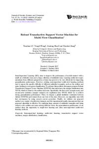
where ri = −yi (f (xi ) + b) is the negative margin and rσ(i) is its sort in the descending order defined in Section 2. The second term in (7) is the average of the negative margins included in the middle interval presented in Figure 1, and it is expressed by the difference of CVaRs at levels ν and µ. The learning algorithm based on this interpretation is proposed in [30] under the name CVaR-(αL , αU )-SVM. The two methods can be shown to be equivalent by setting αL = 1 − ν and αU = 1 − µ. In this paper, the learning algorithm based on (4) is referred to as robust (ν, µ)-SVM to emphasize that it is a robust variant of ν-SVM. TheP representer theorem ensures that the optimal decision function of (4) is represented by 0 f (x) = m i=1 αi k(x, xi ) + b when the kernel function of the RKHS H is given by k(x, x ). As in the case of the standard ν-SVM, the number of support vectors, i.e., the input points xi such that αi 6= 0, is bounded below by (ν − µ)m. In addition, the KKT condition of (4) leads to the fact that any support vector xi satisfies ηi = 1. It is hard to obtain a global optimal solution of (4), since the objective function is nonconvex. As shown in [30, 25], the objective function in (4) is expressed as a difference of convex 5

νm ! 1 rσ(i) (ν − µ)m

frequency prob.

i=µm+1

ri 1−ν

µ

ν−µ

Figure 1: Distribution of negative margins ri = −yi g(xi ), i ∈ [m] for a fixed decision function g(x) = f (x) + b. functions (DC) by using a CVaR representation. Hence, the DC algorithm [28] and convexconcave programming (CCCP) [36] are available to efficiently obtain a stationary point of (4). The same approach is taken by robust C-SVM using the ramp loss [5]. In Algorithm 1, the DC algorithm for robust (ν, µ)-SVM based on the expression (6) is presented. The derivation of the DC algorithm is presented in Appendix A. Algorithm 1 is guaranteed to converge in a finite number of iterations. In the DC algorithm, a monotone decrease of the objective value is generally guaranteed, and in Algorithm 1, the objective value in each iteration is determined by η ∈ Eµ , which can take only a finite number of distinct values. A stationary point is obtained when the objective value is unchanged. The above argument is based on a convergence analysis of robust C-SVM using the ramp loss [5]. In addition, an argument based on polyhedral DC programming shows that the algorithm converges after a finite number of iterations [29]. One can use another stopping rule such that the algorithm terminates when the same η ∈ Eµ is obtained in two consecutive iterations. If the cyclic phenomenon of η is prohibited in some way, convergence in a finite number of iterations is guaranteed.

3.2

Dual Problem and Its Interpretation

The partial dual problem of (4) with a fixed outlier indicator η = (η1 , . . . , ηm ) ∈ Eµ has an intuitive geometric picture. Some variants of ν-SVM can be geometrically interpreted on the basis of the dual form [7, 11, 26]. Substituting (2) into the objective function in (4), we obtain the Lagrangian of problem (4) with a fixed η ∈ Eµ as m m m X 1 X 1 X Lη (α, b, ρ, ξ; β, γ) = αi αj k(xi , xj ) − (ν − µ)ρ + ηi ξi − βi ξi 2 m i,j=1 i=1 i=1  X  m X + γi ρ − ξi − yi k(xi , xj )αj + b , i=1

j

where non-negative slack variables ξi , i ∈ [m] are introduced to represent the hinge loss. Here, the parameters βi and γi for i ∈ [m] are non-negative Lagrange multipliers. For a fixed η ∈ Eµ , 6

Algorithm 1 DC algorithm for robust (ν, µ)-SVM Input: Gram matrix K ∈ Rm×m defined as Kij = k(xi , xj ), i, j ∈ [m], and training labels e ∈ Rm×m is defined as K e ij = yi yj Kij . Let y = (y1 , . . . , ym )T ∈ {+1, −1}m . The matrix K g(x) = f (x) + b be an initial decision function. 1: repeat 2: Compute the sort rσ(1) ≥ · · · ≥ rσ(m) of the negative margin ri = −yi g(xi ), and set ησ(i)

3: 4:

( 0, 1 ≤ i ≤ µm, ← 1, otherwise,

for i ∈ [m]. Let η be (η1 , . . . , ηm )T ∈ Eµ . e m − η)/m and d ← y T (1m − η)/m. Set c ← −K(1 Compute the optimal solution βopt of the problem 1 e + cT β, minm β T Kβ β∈R 2

s. t. 0m ≤ β ≤ 1m /m, β T y = d, β T 1m = ν.

(8)

Set α ← y ◦ (βopt − (1m − η)/m), where ◦ denotes component-wise multiplication of two vectors. P 6: Compute ρ and b using 0 < βi < 1/m =⇒ ρ = yi g(xi ), where g(xi ) = m j=1 Kij αj + b. 7: until the objective value of (4) is unchanged. m X 8: Output: the decision function g(x) = k(x, xi )αi + b. 5:

i=1

the Lagrangian is convex in the parameters α, b, ρ, and ξ and concave in β = (β1 , . . . , βm ) and γ = (γ1 , . . . , γm ). Hence, the min-max theorem [3, Proposition 6.4.3] yields inf

sup Lη (α, b, ρ, ξ; β, γ)

α,b,ρ,ξ β,γ≥0

= sup inf Lη (α, b, ρ, ξ; β, γ) β,γ≥0 α,b,ρ,ξ

X  X   ηi − β i − γi = sup inf ρ γi − (ν − µ) + ξi m β,γ≥0 α,b,ρ,ξ i i X X X 1X αi αj k(xi , xj ) − γi yi k(xi , xj )αj − b yi γ i + 2 i,j i j i

2

X   X X

1 ν−µ ηi

= max − γi yi k(·, xi ) : γi = γi = , 0 ≤ γi ≤ . 2 2 m H i

i:yi =+1

i:yi =−1

Let us give a geometric interpretation of the above expression. For the training data D = {(xi , yi ) : i ∈ [m]}, the convex sets, Uη+ [ν, µ; D] and Uη− [ν, µ; D], are defined as the reduced convex hulls of data points for each label, i.e., Uη± [ν, µ; D]  X X = γi0 k(·, xi ) ∈ H : γi0 = 1, 0 ≤ γi0 ≤ i:yi =±1

i:yi =±1

7

 2ηi for i such that yi = ±1 . (ν − µ)m

The coefficients γi0 , i ∈ [m] in Uη± [ν, µ; D] are bounded above by a non-negative real number that is usually less than one. Hence, the reduced convex hull is a subset of the convex hull of the data points in the RKHS H. Each reduced convex hull is regarded as the domain of the input samples of each label. Accordingly, let Vη [ν, µ; D] be the Minkowski difference of two subsets, Vη [ν, µ; D] = Uη+ [ν, µ; D] Uη− [ν, µ; D], where A B of subsets A and B denotes {a − b : a ∈ A, b ∈ B}. Eventually, for each η ∈ Eµ , the optimal value in the above is represented by inf

sup Lη (α, b, ρ, ξ; β, γ) = −

α,b,ρ,ξ β,γ≥0

 (ν − µ)2 min kf k2H : f ∈ Vη [ν, µ; D] . 8

Hence, the optimal value of (4) is −(ν − µ)2 /8 × opt(ν, µ; D), where opt(ν, µ; D) = max

min

η∈Eµ f ∈Vη [ν,µ;D]

kf k2H .

(9)

Therefore, the dual form of robust (ν, µ)-SVM is expressed as the maximization of the minimum distance between two reduced convex hulls, Uη+ [ν, µ; D] and Uη− [ν, µ; D]. The estimated decision function in robust (ν, µ)-SVM is provided by the optimal solution of (9) up to a scaling factor depending on ν − µ. Moreover, the optimal value is proportional to the squared RKHS norm of the function f (x) ∈ H in the decision function g(x) = f (x) + b.

4 4.1

Breakdown Point of Robust (ν, µ)-SVM Finite-Sample Breakdown Point

Let us describe how to evaluate the robustness of learning algorithms. There are a number of robustness measures for evaluating the stability of estimators. For example, the influence function evaluates the infinitesimal bias of the estimator caused by a few outliers included in the training samples. The gross error sensitivity is the worst-case infinitesimal bias defined with the influence function [12]. In this paper, we use the finite-sample breakdown point, and it will be referred to as the breakdown point for short. The breakdown point quantifies the degree of impact that the outliers have on the estimators when the contamination ratio is not necessarily infinitesimal [8]. In this section, we present an exact evaluation of the breakdown point of robust (ν, µ)-SVM. The breakdown point indicates the largest amount of contamination such that the estimator still gives information about the non-contaminated data [12, Chap.3.2]. More precisely, for an estimator θD based on a dataset D of size m that takes a value in a normed space, the finite-sample breakdown point is defined as ε∗ =

max { κ/m : θD0 is uniformly bounded for D0 ∈ Dκ },

κ=0,1,...,m

where Dκ is the family of datasets of size m including at least m − κ elements in common with the non-contaminated dataset D, i.e.,  Dκ = D0 = {(x0i , yi0 ) : i ∈ [m]} ⊂ X × {+1, −1} : |D0 ∩ D| ≥ m − κ . 8

For simplicity, the dependency of Dκ on the data set D is dropped. The condition of the breakdown point ε∗ can be rephrased as sup kθD0 k < ∞,

D0 ∈Dκ

where k · k is the norm on the normed space. In most cases of interest, ε∗ does not depend on the dataset D. For example, the breakdown point of the one-dimensional median estimator is ε∗ = b(m − 1)/2c/m. To start with, let us derive a lower bound of the breakdown point for the optimal value of problem (4) that is expressed as opt(ν, µ; D) up to a constant factor. As shown in Section 3.2, the boundedness of opt(ν, µ; D) is equivalent to the boundedness of the RKHS norm of f ∈ H in the estimated decision function g(x) = f (x)+b. Given a labeled dataset D = {(xi , yi ) : i ∈ [m]}, let us define the label ratio r as r=

1 min{ |{i : yi = +1}|, |{i : yi = −1}| }. m

Theorem 1. Let D be a labeled dataset of size m with a positive label ratio r. For the parameters ν, µ such that 0 ≤ µ < ν < 1 and νm, µm ∈ N, we assume µ < r/2. Then, the following two conditions are equivalent. (i) The inequality ν − µ ≤ 2(r − 2µ)

(10)

holds. (ii) Uniform boundedness, sup{opt(ν, µ; D0 ) : D0 ∈ Dµm } < ∞ holds, where Dµm is the family of contaminated datasets defined from D. The proof is given in Appendix B.1. The inequality µ < r/2 is a requisite condition. If this inequality is violated, the majority of, say, positive labeled samples in the non-contaminated training dataset can be replaced with outliers. In such a situation, the statistical features in the original dataset will not be retained. Indeed, if µ ≥ r/2 holds, opt(ν, µ; D0 ) is unbounded over D0 ∈ Dµm regardless of ν. Since it is proved by a rigorous description of the above intuitive interpretation, the proof is omitted. Theorem 1 indicates that the breakdown point of the RKHS element in the estimated decision function is greater than or equal to µ, if µ and ν satisfy inequality (10). Conversely, if the inequality ν − µ ≤ 2(r − 2µ) is violated, the breakdown point of robust (ν, µ)-SVM does not reach µ, even though µm samples are removed from the training data. In addition, the inequality (10) indicates the trade-off between the ratio of outliers µ and the ratio of support vectors ν − µ. This result is reasonable. The number of support vectors corresponds to the dimension of the statistical model. When the ratio of outliers is large, a simple statistical model should be used to obtain robust estimators. If there is no outlier in training data, i.e., µ = 0, inequality (10) reduces to ν ≤ 2r. For the standard ν-SVM, this is a necessary and sufficient condition for the optimization problem (1) to be bounded [7]. When the contamination ratio in a training dataset is greater than µ, the estimated decision function is not necessarily bounded. 9

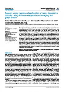
Theorem 2. Suppose that ν and µ are rational numbers such that 0 < µ < 1/4 and µ < ν < 1. Then, there exists a dataset D of size m with the label ratio r such that µ < r/2 and sup{opt(ν, µ; D0 ) : D0 ∈ Dµm+1 } = ∞ hold, where Dµm+1 is defined from D. The proof is given in Appendix B.2. Theorems 1 and 2 lead to the fact that the breakdown point of the function part f ∈ H in the estimated decision function g = f + b is exactly equal to ε∗ = µ, when the learning parameters of the robust (ν, µ)-SVM satisfy µ < r/2 and ν − µ ≤ 2(r − 2µ). Otherwise, the breakdown point of f is strictly less than µ. We show the robustness of the bias term b. Let bD be the estimated bias parameter obtained by robust (ν, µ)-SVM from the training dataset D. We will derive a lower bound of the breakdown point of the bias term. Then, we will show that the breakdown point of robust (ν, µ)-SVM with a bounded kernel is given by a simple formula. Theorem 3. Let D be an arbitrary dataset of size m with a positive label ratio r. Suppose that ν and µ satisfy 0 < µ < ν < 1, νm, µm ∈ N, and µ < r/2. For a non-negative integer `, we assume   ` 0≤2 µ− < ν − µ < 2(r − 2µ). (11) m Then, uniform boundedness sup{ |bD0 | : D0 ∈ Dµm−` } < ∞ holds, where Dµm−` is defined from D. The proof is given in Appendix B.3. Note that the inequality (11) is a sufficient condition of inequality (10). Theorem 3 guarantees that the breakdown point of the estimated decision function f + b is not less than µ − `/m when (11) holds. When the kernel function is bounded, the boundedness of the function part f ∈ H in the decision function f + b almost guarantees the boundedness of the bias term b. Theorem 4. Let D be an arbitrary dataset of size m with a positive label ratio r. For the parameters ν, µ such that 0 < µ < ν < 1 and νm, µm ∈ N, suppose that µ < r/2 and ν − µ < 2(r − 2µ) hold. In addition, assume that the kernel function k(x, x0 ) of the RKHS H is bounded, i.e., supx∈X k(x, x) < ∞. Then, uniform boundedness, sup{ |bD0 | : D0 ∈ Dµm } < ∞, holds, where Dµm is defined from D. The proof is given in Appendix B.4. Compared with Theorem 3 in which arbitrary kernel functions are treated, Theorem 4 ensures that a tighter lower bound of the breakdown point is obtained for bounded kernels. The above result agrees with those of other studies. The authors of [34] proved that bounded kernels produce robust estimators for regression problems in the sense of bounded response, i.e., robustness against a single outlier. Combining Theorems 1, 2, 3 and 4, we find that the breakdown point of (ν, µ)-SVM with µ < r/2 is given as follows. 10

Unbounded kernel ratio of support vectors: ν − µ

ratio of support vectors: ν − µ

Bounded kernel 2r ε∗ < µ ε∗ = µ

2r ε∗ < µ ε∗ = µ

2r/3

0 0

ratio of removed samples: µ

0 0

r/2

∗ ≤µ ≤ε ∗ ≤µ m ε / 1 µ − 2/m ≤ − µ ... ∗ ≤µ ≤ε m / 1

r/3 ratio of removed samples: µ

r/2

Figure 2: Left (resp. Right) panel: breakdown point of (f, b) ∈ H×R given by robust (ν, µ)-SVM with bounded (resp. unbounded) kernel. Bounded kernel: For ν − µ > 2(r − 2µ), the breakdown point of f ∈ H is less than µ. For ν − µ ≤ 2(r − 2µ), the breakdown point of (f, b) ∈ H × R is equal to µ. Unbounded kernel: For ν − µ > 2(r − 2µ), the breakdown point of f ∈ H is less than µ. For 2µ < ν − µ ≤ 2(r − 2µ), the breakdown point of (f, b) ∈ H × R is equal to µ. When 0 < ν − µ < min{2µ, 2(r − 2µ)}, the breakdown point of the function part f is equal to µ, and the breakdown point of the bias term b is bounded from below by µ − `/m and from above by µ, where ` ∈ N depends on ν and µ, as shown in Theorem 3. Figure 2 shows the breakdown point of robust (ν, µ)-SVM. The line ν − µ = 2(r − 2µ) is critical. For unbounded kernels, we obtain only a bound of the breakdown point. Hence, there is a possibility that unbounded kernels provide the same breakdown point as bounded kernels.

4.2

Acceptable Region for Learning Parameters

The theoretical analysis in Section 4.1 suggests that robust (ν, µ)-SVM satisfying 0 < ν − µ < 2(r − 2µ) is a good choice for obtaining a robust classifier, especially when a bounded kernel is used. Here, r is the label ratio of the non-contaminated original data D, and usually it is unknown in real-world data analysis. Thus, we need to estimate r from the contaminated dataset D0 . If an upper bound of the outlier ratio is known to be µ ¯, we have D0 ∈ Dµ¯m , where Dµ¯m is 0 0 defined from D. Let r be the label ratio of D . Then, the label ratio of the original dataset D should satisfy rlow ≤ r ≤ rup , where rlow = max{r0 − µ ¯, 0} and rup = min{r0 + µ ¯, 1/2}. Let Λlow and Λup be Λlow = {(ν, µ) : 0 ≤ µ ≤ µ ¯, 0 < ν − µ < 2(rlow − 2µ)}, Λup = {(ν, µ) : 0 ≤ µ ≤ µ ¯, 0 < ν − µ < 2(rup − 2µ)}. Then, robust (ν, µ)-SVM with (ν, µ) ∈ Λlow reaches the breakdown point µ for any noncontaminated dataset D such that D0 ∈ Dµm for given D0 . On the other hand, the parameters (ν, µ) on the outside of Λup is not necessary. Indeed, the parameter µ such that 0 < µ ≤ µ ¯ is 0 sufficient to detect outliers. In addition, for any non-contaminated data D such that D ∈ Dµ¯m 11

for given D0 , (ν, µ) satisfying ν − µ > 2(rup − 2µ) does not yield a learning method that reaches the breakdown point µ. When an upper bound µ ¯ is unknown, we use µ ¯ = r/2 and obtain r¯low ≤ r ≤ r¯up , where r¯low = 2r0 /3 and r¯up = min{2r0 , 1/2}. Hence, in the worst case, the admissible set of the learning parameters ν and µ is given as Λlow = {(ν, µ) : 0 < ν − µ < 2(¯ rlow − 2µ)}, Λup = {(ν, µ) : 0 < ν − µ < 2(¯ rup − 2µ)}.

(12)

Given contaminated training data D0 , for any D of size m with a label ratio r ∈ [¯ rlow , r¯up ] such that D0 ∈ Dµm with µ < r¯low /2, robust (ν, µ)-SVM with (ν, µ) ∈ Λlow provides a classifier with the breakdown point µ. The parameter (ν, µ) on the outside of Λup is not necessary for the same reasons as for Λup . The acceptable region of (ν, µ) is useful when the parameters are determined by a grid search based on cross validation. The numerical experiments presented in Section 6 applied a grid search to the region Λup .

5

Asymptotic Properties

Let us consider the asymptotic properties of robust (ν, µ)-SVM. In the literature [17], a uniform bound of the generalization ability of the standard ν-SVM was calculated for the case that the class of classifiers is properly constrained such that the bias term in the decision function is bounded in advance. Moreover, in [22], the asymptotic properties of ν-SVM with an unconstrained parameter space were investigated for a fixed ν. To our knowledge, however, the statistical consistency of ν-SVM has not yet been proved. The main difficulty comes from the fact that the loss function −νρ + [ρ − yg(x)]+ in (1) is not bounded from below. Here, therefore, we will study the statistical asymptotic properties of robust (ν, µ)-SVM on the basis of the classical asymptotic theory of L-estimators [19, 23]. Given a training dataset, the loss function of the robust (ν, µ)-SVM for a fixed decision function g(x) = f (x) + b is given by (7). The sort of the negative margins, r(1) ≥ · · · ≥ rσ(m) for ri = −yi g(xi ), i ∈ [m] is called the order statistics, and the linear sum of the order statistics is called the L-estimator. The asymptotic properties of L-estimators have been investigated in the field of mathematical statistics (see [31, Chap. 22], [19, Chap. 8] and references therein for details). We will derive the asymptotic distribution of (7) with reference to [23]. Let us define Fg (r) as the distribution function of the random variable Rg = −Y g(X), in which (X, Y ) is generated from the population distribution of the training samples. Furthermore, the distribution function Gg (r) is defined as the conditional probability, Gg (r) = Pr{Rg ≤ r | q¯1−ν ≤ Rg < q 1−µ }, where q¯1−ν and q 1−µ are quantiles defined as q¯1−ν = sup{r : Fg (r) ≤ 1 − ν},

q 1−µ = inf{r : Fg (r) ≥ 1 − µ}, 12

target density

Bµ outlier density

q 1−ν q 1−µ Figure 3: Probability density consisting of two components: the target density and outlier density. The gap between two components is the 1 − µ quantile of the length Bµ .

for 0 < µ < ν < 1. The mean value under the distribution Gg is denoted as eg , i.e., eg = E[Rg | q¯1−ν ≤ Rg < q 1−µ ], which is nothing but a trimmed mean of Rg . In addition, let Tm be Tm

1 = (ν − µ)m

νm X

r(i) . i=µm+1

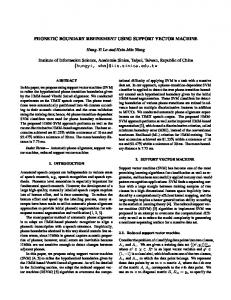
√ According to [23], the asymptotic distribution of m(Tm −eg ) is expressed by a transformation of a three-dimensional normal distribution. Hence, the random variable Tm converges in probability to eg . We omit the detailed definition of the asymptotic distribution of Tm (see [23]). √ The asymptotic distribution of m(Tm − eg ) has an interesting property. Suppose that √ m(Tm − eg ) converges in law to a random variable Zg , that is distributed from the above asymptotic distribution. Let Bµ be the length of the interval Fg−1 (1 − µ), as shown in Figure 3. When the probability density of Fg is strictly positive, Bµ equals zero. In addition, suppose that the length of the interval Fg−1 (1 − ν) is zero. Then, the mean value of Zg can be expressed as p Bµ µ(1 − µ) E[Zg ] = √ , 2π(ν − µ)

as shown in [23]. As a result, the trimmed mean of the negative margins in (7) is asymptotically represented as     νm X Bµ 1 1 (ν − µ) · rσ(i) = (ν − µ)eg + O √ + Op √ , (ν − µ)m m m i=µm+1

where Op (·) is the probabilistic order defined in [31, Chap. 2]. The above equation is a pointwise approximation at each (f, b) ∈ H × R. In light of the above argument, let us consider the statistical properties of robust (ν, µ)-SVM. Robust (ν, µ)-SVM in (4) and ROD in (5) can be made equivalent by appropriately setting the learning parameters ν, µ and λ, where the outlier indicator η in ROD can take any real number in [0, 1]m . The discussion in [33] on setting the parameter µ in ROD is based on the following observation. When µ is small, most ηi ’s take one, and the rest take zero, while, for large µ, all values of η fall below one. This phenomenon is called the second order phase transition in the 13

maximal value of η. The authors reported that the phase transition occurs at the value of µ that corresponds to the true ratio of outliers. The above observation is plausible. Let us consider robust (ν, µ)-SVM with η ∈ [0, 1]m that corresponds to ROD with the learning parameters λ and µ. Suppose that the probability density of the negative margin, Fg (r), is separated into two components as shown in Fig. 3 and that the true outlier ratio is µ0 . When µ is less than µ0 , there are still some outliers that have not been removed from the training data. Hence, negative margins ri , i ∈ [m] can take a wide range of real values, and a tie will not occur. As a result, the outlier indicator ηi tends to take only zero or one, even when ηi can take a real number in the interval [0, 1]. If µ is larger than µ0 , all outliers can be removed from the training data. In such a case, q 1−ν and q 1−µ will be close to each other, and some negative margins ri with ηi > 0 will concentrate around q 1−µ . If some negative margins take exactly the same value, the outlier indicators on those samples can take real values in the open interval (0, 1). Since ROD solves a semidefinite relaxation of the non-convex problem, it is conceivable that the numerical solution η in ROD will have a similar feature even if the negative margins do not take exactly the same value.

6

Numerical Experiments

We conducted numerical experiments on synthetic and benchmark datasets to compare some variants of SVMs. The DC algorithm was used to obtain a classifier in the case of robust (ν, µ)SVM and robust C-SVM using the ramp loss. The DC algorithm for robust C-SVM is presented in [5]. We used CPLEX to solve the convex quadratic problems.

6.1

Breakdown Point

Let us consider the validity of inequality (10) in Theorem 1. In the numerical experiments, the original data D was generated using mlbench.spirals in the mlbench library of the R language [14]. Given an outlier ratio µ, positive samples of size µm were randomly chosen from D, and they were replaced with randomly generated outliers to obtain a contaminated dataset D0 ∈ Dµm . The original data D and an example of the contaminated data D0 ∈ Dµm are shown in Fig. 4. The decision function g(x) = f (x) + b was estimated from D0 by using robust (ν, µ)-SVM. Here, the true outlier ratio µ was used as the parameter of the learning algorithm. The norms of f and b were then evaluated. The above process was repeated 30 times for each parameters (ν, µ), and the maximum value of kf kH and |b| was computed. Figure 5 shows the results of the numerical experiments. The maximum norm of the estimated decision function is plotted for the parameter (µ, ν − µ) on the same axis as Fig. 2. The top (bottom) panels show the results for a Gaussian (linear) kernel. The left and middle columns show the maximum norm of f and b, respectively. The maximum test errors are presented in the right column. In all panels, the red points denote the top 50 percent of values, and the asterisk (∗) is the point that violates the inequality ν − µ ≤ 2(r − 2µ). In this example, the numerical results agree with the theoretical analysis in Section 4; i.e., the norm becomes large when the inequality ν − µ ≤ 2(r − 2µ) is violated. Accordingly, the test error gets close to 0.5— no information for classification. Even when the unbounded linear kernel is used, robustness is confirmed for the parameters in the left lower region in the right panel of Fig. 2.

14

example of D0 ∈ Dµm

4 2 0 -2

-2

0

2

4

original data D

-2

-1

0

1

2

3

4

-2

-1

0

1

2

3

4

Figure 4: The left panel shows the original data D, and the right panel shows the contaminated data D0 ∈ Dµm . In this example, the sample size is m = 200, and the outlier ratio is µ = 0.1. In the bottom right panel, the test error gets large when the inequality ν − µ ≤ 2(r − 2µ) holds. This result comes from the problem setup. Even with non-contaminated data, the test error of the standard ν-SVM is approximately 0.5, because the linear kernel works poorly for spiral data. Thus, the worst-case test error can go beyond 0.5. For the parameter at which (10) is violated, the test error is always close to 0.5. Thus, a learning method with such parameters does not provide any useful information for classification.

6.2

Prediction Accuracy

We compared the generalization ability of the robust (ν, µ)-SVM with existing classifiers such as standard ν-SVM and robust C-SVM using the ramp loss. The datasets are presented in Table 1. All the datasets are provided in the mlbench and kernlab libraries of the R language [14]. In all the datasets, the number of positive samples is less than or equal to that of negative samples. Before running the learning algorithms, we standardized each input variable with mean zero and standard deviation one. We randomly split the dataset into training and test sets. To evaluate the robustness, the training data was contaminated by outliers. More precisely, we randomly chose positive labeled samples in the training data and changed their labels to negative; i.e., we added outliers by flipping the labels. After that, robust (ν, µ)-SVM, robust C-SVM using the ramp loss, and the standard ν-SVM were used to obtain classifiers from the contaminated training dataset. The prediction accuracy of each classifier was then evaluated over test data that had no outliers. Linear and Gaussian kernels were employed for each learning algorithm. The learning parameters, such as µ, ν, and C, were determined by conducting a grid search based on five-fold cross validation over the training data. For robust (ν, µ)-SVM, the parameter (µ, ν) was selected from the region Λup in (12). For standard ν-SVM, the candidate of the regularization parameter ν was selected from the interval (0, 2r0 ), where r0 is the label ratio of the contaminated training data. For robust C-SVM, the regularization parameter C was selected from the interval [10−7 , 107 ]. In the grid search of the parameters, 24 or 25 candidates were examined for each learning method. Thus, we needed to solve convex or non-convex optimization 15

test error

log10 |b|

log10 ∥f ∥H

(a) Gaussian kernel

1

-0.5 -1.0

0

-1.5

-1

-2.0

-2

0.55 0.50 0.45 0.40 0.35

-3

-2.5 1.0 -3.0

0.8

-4

-3.5 -4.0 0.05

0.2 0.10

0.15

0.20

ν−

0.0 0.25

1.0

0.8

0.6 0.4

0.30

1.0

0.25

0.6 -5

µ

0.4 0.2

-6 0.05

0.10

µ

0.15

0.20

ν−

0.0 0.25

0.8 0.6 0.4

0.20

µ

0.15 0.05

0.2 0.10

µ

plot of log10 kf kH

0.15

0.20

ν−

0.0 0.25

µ

µ

plot of log10 |b|

plot of test error

2

test error

log10 |b|

log10 ∥f ∥H

(b) Linear kernel

0

0

0.65

-2 -2

0.60 -4 1.0

-4 1.0

-6

1.0 -6

0.8 0.6 0.4

-8 0.2 -10 0.05

0.10

0.15

0.20

0.0 0.25

µ

plot of log10 kf kH

ν−

0.55

0.8

0.8

0.6

0.6 -8

µ

0.2 -10 0.05

0.10

0.15

0.20

0.0 0.25

µ

0.4

0.50

0.4

ν−

µ

0.2 0.45 0.05

0.10

0.15

0.20

0.0 0.25

ν−

µ

µ

plot of log10 |b|

plot of test error

Figure 5: Plots of the maximum norms and the worst-case test errors. The top (Bottom) panels show the results for a Gaussian (linear) kernel. Red points mean the top 50 percent of values, and the asterisk (∗) is the point that violates the inequality ν − µ ≤ 2(r − 2µ).

16

problems more than 24 × 5 times in order to obtain a classifier. The above process was repeated 30 times, and the average test error was calculated. The results are presented in Table 1. For non-contaminated training data, robust (ν, µ)-SVM and robust C-SVM were comparable to the standard ν-SVM. When the outlier ratio is high, we can conclude that robust (ν, µ)-SVM and robust C-SVM tend to work better than the standard νSVM. In this experiment, the kernel function does not affect the relative prediction performance of these learning methods. In large datasets such as spam and Satellite, robust (ν, µ)-SVM tends to outperform robust C-SVM. When learning parameters, such as ν, µ, and C, are appropriately chosen by using a large dataset, learning algorithms with plural learning parameters clearly work better than those with a single learning parameter. In addition, in robust C-SVM, there is a difficulty in choosing the regularization parameter. Indeed, the parameter C does not have a clear meaning, and thus, it is not straightforward to determine the candidates of C in the grid search optimization. In contrast, the parameter ν in ν-SVM and its robust variant has a clear meaning, i.e., a lower bound of the ratio of support vectors and an upper bound of the margin error on the training data [17]. Such clear meaning is of great help to choose candidate points of regularization parameters. We conducted another experiment in which the learning parameters ν, µ and C were determined using only one validation set, i.e., non-cross validation (the details are not presented here). The dataset was split into training, validation and test sets. The learning parameters, ν, µ, and C, that minimized the prediction error on the validation set were selected. This method greatly reduced the computational cost of the cross validation. However, robust (ν, µ)-SVM did not necessarily produce a better classifier compared with the other methods. Since robust (ν, µ)-SVM has two learning parameters, we need to carefully select them using cross validations rather than simple validations in order to achieve high prediction accuracy.

7

Concluding Remarks

We presented robust (ν, µ)-SVM and studied its statistical properties. The robustness property was analyzed by computing the exact breakdown point. As a result, we obtained inequalities for the learning parameters ν and µ that guarantee the robustness of the learning algorithm. The statistical theory of the L-estimator was then used to investigate the asymptotic behavior of the classifier. Numerical experiments showed that the inequalities are critical to obtaining a robust classifier. The prediction accuracy of the proposed method was numerically compared with those of other methods, and it was found that the proposed method with carefully chosen learning parameters delivers more robust classifiers than those of other methods such as standard ν-SVM and robust C-SVM using the ramp loss. In the future, we will explore the robustness properties of more general learning methods. Another important issue is to develop efficient optimization algorithms. Although the DC algorithm [5, 28] and convex relaxation [33, 34] are promising methods, more scalable algorithms will be required to deal with massive datasets that are often contaminated by outliers.

17

Table 1: Test error and standard deviation of robust (ν, µ)-SVM, robust C-SVM and ν-SVM. The dimension of the input vector, the number of training samples, the number of test samples, and the label ratio of all samples with no outliers are shown for each dataset. Linear and Gaussian kernels were used to build the classifier in each method. The outlier ratio in the training data ranged from 0% to 15%, and the test error was evaluated on the non-contaminated test data. The asterisk (∗) means the best result for a fixed kernel function in each dataset, and the double asterisks (∗∗) mean that the corresponding method is 5% significant compared with the second best method under a one-sided t-test. The learning parameters were determined by five-fold cross validation on the contaminated training data. Sonar: dim x = 60, #train=104, #test=104, r = 0.466. Linear kernel Gaussian kernel robust robust robust robust (ν, µ)-SVM C-SVM ν-SVM (ν, µ)-SVM C-SVM ν-SVM outlier 0% .258(.032) .270(.038) *.256(.051) *.179(.038) .188(.043) .181(.039) 5% *.256(.039) .273(.047) .258(.046) .225(.042) .229(.051) *.224(.061) 10% *.297(.060) .306(.067) .314(.060) .249(.059) **.230(.046) .259(.062) 15% *.329(.061) .339(.064) .345(.062) .280(.053) *.280(.050) .294(.064) BreastCancer: dim x = 10, #train=350, #test=349, r = 0.345. Linear kernel Gaussian kernel robust robust robust robust outlier (ν, µ)-SVM C-SVM ν-SVM (ν, µ)-SVM C-SVM 0% .033(.010) .035(.008) *.033(.006) *.032(.008) .035(.012) 5% .034(.009) *.034(.010) .043(.015) *.032(.005) .033(.007) 10% .055(.015) *.051(.026) .076(.036) **.035(.008) .043(.025) 15% .136(.058) *.120(.050) .148(.058) .160(.083) *.145(.070)

ν-SVM .033(.010) .033(.006) .038(.008) .150(.110)

PimaIndiansDiabetes: dim x = 8, #train=384, #test=384, r = 0.349. Linear kernel Gaussian kernel robust robust robust robust outlier (ν, µ)-SVM C-SVM ν-SVM (ν, µ)-SVM C-SVM 0% .237(.018) *.232(.014) .246(.018) *.238(.021) .240(.019) 5% .239(.019) *.237(.016) .269(.036) *.264(.025) .267(.024) 10% **.280(.046) .299(.042) .330(.030) .302(.039) *.293(.036) 15% **.338(.042) .349(.030) .351(.026) *.344(.028) .344(.031)

ν-SVM .243(.022) .273(.024) .315(.038) .353(.016)

spam: dim x = 57, #train=1000, #test=3601, r = 0.394. Linear kernel Gaussian kernel robust robust robust robust outlier (ν, µ)-SVM C-SVM ν-SVM (ν, µ)-SVM C-SVM ν-SVM 0% .083(.005) .088(.006) *.083(.005) .081(.005) .086(.006) *.081(.006) 5% **.094(.008) .104(.013) .109(.010) .095(.008) .097(.009) *.095(.008) 10% **.129(.022) .152(.020) .166(.067) *.129(.015) .133(.017) .141(.030) 15% **.201(.029) .240(.030) .256(.091) **.206(.018) .223(.030) .240(.055) Satellite: dim x = 36, #train=2000, #test=4435, r = 0.234. Linear kernel Gaussian kernel robust robust robust robust outlier (ν, µ)-SVM C-SVM ν-SVM (ν, µ)-SVM C-SVM ν-SVM 0% .097(.004) .096(.003) **.094(.003) .069(.031) .067(.004) **.063(.004) 5% .101(.003) *.100(.005) .100(.004) *.072(.015) .078(.007) .078(.043) 10% **.148(.020) .161(.026) .161(.019) *.117(.034) .126(.040) .137(.027)

18

A

Derivation of DC Algorithm

According to (6), the objective function of the robust (ν, µ)-SVM is expressed as Φ(α, b, ρ) = ψ0 (α, b, ρ) − ψ1 (α, b) using the convex functions ψ0 and ψ1 defined as m

1 1 X ψ0 (α, b, ρ) = αT Kα − νρ + [ρ + ri ], 2 m i=1

ψ1 (α, b) = max

η∈Eµ

1 m

m X i=1

(1 − ηi )ri ,

P m×m is the Gram matrix where ri is the negative margin ri = −yi ( m i=1 Kij αi + b) and K ∈ R defined by Kij = k(xi , xj ), i, j ∈ [m]. Let αt , bt , ρt be the solution obtained after t iterations of the DC algorithm. Then, the solution is updated to the optimal solution of min ψ0 (α, b, ρ) − uT α − vb, α,b,ρ

(13)

where (u, v) ∈ Rm+1 with u ∈ Rm , v ∈ R is an element of the subgradient of ψ1 at (αt , bt ). The subgradient of ψ1 is given as ∂ψ1 (αt , bt )  1 1 = conv (u, v) : u = − K(y ◦ (1m − η)), v = − y T (1m − η), m m

 where η is a maximum solution of the problem in ψ1 (αt , bt ) ,

where convS denotes the convex hull of the set S. As shown in Algorithm 1, a parameter η that meets the condition in the above subgradient is obtained from the sort of the negative margin of the decision function defined from (αt , bt ). The dual problem of (13) is presented in (8), up to a constant term that is independent of the optimization parameter.

B B.1

Proofs of Theorems Proof of Theorem 1

The proof is decomposed into two lemmas. Lemma 1 shows that condition (i) is sufficient for condition (ii), and Lemma 2 shows that condition (ii) does not hold if inequality (10) is violated. For the dataset D = {(xi , yi ) : i ∈ [m]}, let I+ and I− be the index sets defined as I± = {i : yi = ±1}. When the parameter µ is equal to zero, the theorem holds according to the argument on the standard ν-SVM [7]. Below, we assume µ > 0. Lemma 1. Under the assumptions of Theorem 1, condition (i) leads to condition (ii). Proof of Lemma 1. We show that Vη [ν, µ; D0 ] is not empty for any D0 ∈ Dµm . For a parameter µ such that µ < r/2, let c > 0 be a positive constant satisfying µ = r/(c + 2). Then, (10) is expressed as ν ≤ (r + 2cr)/(c + 2). For a contaminated dataset D0 = {(x0i , yi0 ) : i ∈ [m]} ∈ Dµm , let us define Ie+ ⊂ I+ as an index set such that (xi , yi ) ∈ D for i ∈ Ie+ is replaced with (x0i , yi0 ) ∈ D0 19

as an outlier. In the same way, Ie− ⊂ I− is defined for negative samples in D. Therefore, for any index i in I+ \ Ie+ or I− \ Ie− , we have (xi , yi ) = (x0i , yi0 ). The assumptions of the theorem ensure |Ie+ | + |Ie− | ≤ µm. From µm = min{|I+ |, |I− |}/(c + 2), we obtain |Ie+ | ≤ |I+ |/(c + 2) < (c + 1)|I+ |/(c + 2) ≤ |I+ \ Ie+ |, |Ie− | ≤ |I− |/(c + 2) < (c + 1)|I− |/(c + 2) ≤ |I− \ Ie− |.

Given η ∈ Eµ , the sets Ueη+ [ν, µ; D0 ] and Ueη− [ν, µ; D0 ] are defined by Ueη± [ν, µ; D0 ]  X = γi0 k(·, x0i ) ∈ H : i:yi0 =±1

X

γi0 i:yi0 =±1

= 1, 0 ≤

γi0

 2ηi 0 e , γi = 0 for i 6∈ I± \ I± . ≤ (ν − µ)m

Note that Ueη± [ν, µ; D0 ] ⊂ Uη± [ν, µ; D0 ] holds because of the additional constraint, γi0 = 0 for i 6∈ I± \ Ie± . In addition, we have Ueη± [ν, µ; D0 ] ⊂ conv{k(·, xi ) : i ∈ I± }, since only the element k(·, x0i ) with i ∈ I± \ Ie± , i.e. x0i = xi , can have a non-zero coefficient γi0 in Ueη± [ν, µ; D0 ]. We prove that Ueη+ [ν, µ; D0 ] and Ueη− [ν, µ; D0 ] are not empty. The size of the index sets {i ∈ I± \ Ie± : ηi = 1} is bounded below by c|I± | (c + 1)|I± | − µm ≥ > 0. |{i ∈ I± \ Ie± : ηi = 1}| ≥ c+2 c+2

The inequality ν − µ ≤ 2(r − 2µ) is equivalent to 1 ≤ 2cr/((ν − µ)(c + 2)). Hence, we have 1≤

2cr 2 c|I± | 2 ≤ · ≤ · |{i ∈ I± \ Ie± : ηi = 1}|, (ν − µ)(c + 2) (ν − µ)m c + 2 (ν − µ)m

implying that the sets Ueη± [ν, µ; D0 ] are not empty. Indeed, the coefficients defined by γj0 =

2 1 ≤ e (ν − µ)m |{i ∈ I± \ I± : ηi = 1}|

for j ∈ {i ∈ I± \ Ie± : ηi = 1} and otherwise γj0 = 0 admit all the constraints in Ueη± [ν, µ; D0 ]. eη [ν, µ; D0 ] ⊂ Vη [ν, µ; D0 ], where Since ∅ = 6 Ueη± [ν, µ; D0 ] ⊂ Uη± [ν, µ; D0 ] holds, we have ∅ = 6 V eη [ν, µ; D0 ] = Ueη+ [ν, µ; D0 ] Ueη− [ν, µ; D0 ]. V Now, let us prove the inequality

0 ≤ max max 0

inf

D ∈Dµm η∈Eµ f ∈Vη [ν,µ;D0 ]

kf k2H < ∞.

(14)

The above argument leads to min

f ∈Vη [ν,µ;D0 ]

kf k2H ≤

min eη [ν,µ;D0 ] f ∈V

kf k2H < ∞

for any η ∈ Eµ . Let us define C[D] = conv{k(·, xi ) : i ∈ I+ } conv{k(·, xi ) : i ∈ I− } for the original dataset D. Then, the inclusion relation Ueη± [ν, µ; D0 ] ⊂ conv{k(·, xi ) : i ∈ I± } leads to 20

eη [ν, µ; D0 ] ⊂ C[D]. Hence, we obtain V

opt(ν, µ; D0 ) = max

min

kf k2H

≤ max

min

kf k2H

≤ max

max

η∈Eµ f ∈Vη [ν,µ;D0 ]

η∈Eµ f ∈V eη [ν,µ;D0 ]

η∈Eµ f ∈V eη [ν,µ;D0 ]

kf k2H

≤ max kf k2H f ∈C[D]

< ∞. The boundedness of maxf ∈C[D] kf k2H comes from the compactness of C[D] and the continuity of the norm. More precisely, it is bounded above by twice the maximum eigenvalue of the Gram matrix defined from the non-contaminated data D. The upper bound does not depend on the contaminated dataset D0 ∈ Dµm . Thus, the first inequality of (14) holds. Lemma 2. Under the condition of Theorem 1, we assume ν − µ > 2(r − 2µ). Then, we have sup{opt(µ, ν; D0 ) : D0 ∈ Dµm } = ∞. Proof of Lemma 2. We use the same notation as in the proof of Lemma 1. Without loss of generality, we assume r = |I− |/m. The parameter µ is expressed as µ = r/(c + 2) for c > 0. We prove that there exists a feasible parameter η ∈ Eµ and a contaminated training set D0 = {(x0i , yi0 ) : i ∈ [m]} ∈ Dµm such that Uη− [ν, µ; D0 ] = ∅. The construction of the dataset D0 is illustrated in Figure 6. Suppose that |Ie+ | = 0 and |Ie− | = µm and that yi0 = +1 holds for all i ∈ Ie− , meaning that all outliers in D0 are made by flipping the labels of the negative samples in D. This is possible, because µm < |I− |/2 < |I− | holds. The inequality ν − µ > 2(r − 2µ) leads to 1>

2 c · |I− |. (ν − µ)m c + 2

(15)

0 ) ∈ E is defined by η 0 = 0 for µm samples in I \ Ie , and The outlier indicator η 0 = (η10 , . . . , ηm µ − − i 0 ηi = 1 otherwise. This assignment is possible because

Then, we have

c+1 1 |I− \ Ie− | = |I− | − µm = |I− | > |I− | = µm. c+2 c+2 |{i ∈ I− \ Ie− : ηi0 = 1}| = |I− \ Ie− | − µm = |I− | − 2µm c = |I− |. c+2

From (15) and (16), we have 1>

2 |{i ∈ I− \ Ie− : ηi0 = 1}|. (ν − µ)m 21

(16)

I−

I+

ηi′ = 0

I!− : yi = −1 #→ yi′ = +1

I!+ = ∅

Figure 6: Index sets Ie± and value of ηi0 defined in the proof of Lemma 2. In addition, yi0 = −1 holds only when i ∈ I− \ Ie− . Therefore, we have Uη−0 [ν, µ; D0 ] = ∅. The infeasibility of the dual problem means the unboundedness of the primal problem. Hence, there exists a contaminated dataset D0 ∈ Dµm and an outlier indicator η 0 ∈ Eµ such that opt(µ, ν; D0 ) ≥

min

f ∈Vη0 [ν,µ;D0 ]

kf k2H = ∞

holds.

B.2

Proof of Theorem 2

Proof. For a rational number µ ∈ (0, 1/4), there exists an m ∈ N such that µm ∈ N and 2µm + 1 ≤ m − (2µm + 1) hold. For such m, let D = {(xi , yi ) : i ∈ [m]} be a training data such that |I− | = 2µm + 1 and |I+ | = m − (2µm + 1), where the index sets I± are defined in the proof of Appendix B.1. Since the label ratio of D is r = min{|I− |, |I+ |}/m = 2µ + 1/m, and we have µ < r/2. For Dµm+1 defined from D, let D0 = {(x0i , yi0 ) : i ∈ [m]} ∈ Dµm+1 be a contaminated dataset of D such that µm + 1 outliers are made by flipping the labels of the negative samples in D. Thus, there are µm negative samples in D0 . Let us define the outlier 0 ) ∈ E such that η 0 = 0 for µm negative samples in D 0 . Then, any indicator η 0 = (η10 , . . . , ηm µ i 0 0 sample in D with ηi = 1 should be a positive one. Hence, we have Uη−0 [ν, µ; D0 ] = ∅. The infeasibility of the dual problem means that the primal problem is unbounded. Thus, we obtain opt(ν, µ; D0 ) = ∞.

B.3

Proof of Theorem 3

Let us define fD + bD with fD ∈ H, bD ∈ R as the decision function estimated using robust (ν, µ)-SVM based on the dataset D. Proof. The non-contaminated dataset is denoted as D = {(xi , yi ) : i ∈ [m]}. For the dataset D, let I+ and I− be the index sets defined by I± = {i : yi = ±1}. Under the conditions of Theorem 3, inequality (10) holds. Given a contaminated dataset D0 = {(x0i , yi0 ) : i ∈ [m]} ∈ Dµm−` , let ri0 (b) be the negative margin of fD0 + b, i.e., ri0 (b) = −yi0 (fD0 (x0i ) + b) for (x0i , yi0 ) ∈ D0 . For b ∈ R, the function ζ(b) is defined as ζ(b) =

1 X 0 ri (b), m i∈Tb

22

where the index set Tb is given by Tb = {σ(j) ∈ [m] : µm + 1 ≤ j ≤ νm} 0 0 for the sorted negative margins, rσ(1) (b) ≥ · · · ≥ rσ(m) (b). For simplicity, we drop the dependency of the permutation σ on b. The estimated bias term bD0 is the optimal solution of ζ(b) because of (7). The function ζ(b) is continuous. In addition, ζ(b) is linear on the interval such that Tb is unchanged. Hence, ζ(b) is a continuous piecewise linear function. Below, we prove that the minimum solution of ζ(b) is bounded regardless of the contaminated dataset D0 ∈ Dµm−` .

For the non-contaminated data D, let R be a positive real number such that sup{|fD00 (x)| : (x, y) ∈ D, D00 ∈ Dµm−` } ≤ R. The existence of R is guaranteed. Indeed, one can choose p R= sup kfD00 kH · max k(x, x) < ∞, (x,y)∈D

D00 ∈Dµm−`

because the RKHS norm of fD00 is uniformly bounded above for D00 ∈ Dµm−` and D is a finite set. For the contaminated dataset D0 = {(x0i , yi0 ) : i ∈ [m]} ∈ Dµm−` , let us define the index 0 0 , I0 sets I± in,± and Iout,± for each label by 0 I± = {i ∈ [m] : yi0 = ±1},

0 0 Iin,± = {i ∈ I± : |fD0 (x0i )| ≤ R},

0 0 Iout,± = {i ∈ I± : |fD0 (x0i )| > R}.

For any non-contaminated sample (xi , yi ) ∈ D, we have |fD0 (xi )| ≤ R. Hence, (x0i , yi0 ) ∈ D0 for 0 should be an outlier that is not included in D. This fact leads to i ∈ Iout,± 0 0 |Iout,+ | + |Iout,− | ≤ µm − `,

0 |Iin,± | ≥ |I± | − (µm − `) ≥ (r − µ)m + `.

Based on the argument above, we prove two propositions: 1. The function ζ(b) is increasing for b > R. 2. The function ζ(b) is decreasing for b < −R. In addition, for any D0 ∈ Dµm−` , the Lipschitz constant of ζ(b) is greater than or equal to 1/m for R < |b|. Let us prove the first statement. If b > R holds, we have 0 R − b < min{ri0 (b) : i ∈ Iin,− }

(17)

0 from the definition of the index set Iin,− . Let us consider two cases: (i) for all i ∈ Tb , R−b < ri0 (b) holds, and (ii) there exists an index i ∈ Tb such that ri0 (b) ≤ R − b.

0 ∩T , For a fixed b such that b > R, let us assume (i) above. Then, for any index i in I+ b 0 0 ∩ T is less we have R < −fD0 (x0i ), meaning that i ∈ Iout,+ . Hence, the size of the set I+ b 0 ∩ T is greater than or equal to than or equal to µm − `. Therefore, the size of the set I− b

23

(ν −µ)m−(µm−`) = (ν −2µ)m+`. The first inequality of (11) leads to (ν −2µ)m+` > µm−`. Therefore, in the set Tb , the number of negative samples is more than the number of positive samples. For a fixed b such that b > R, let us assume (ii) above. Due to the inequality (17), for any 0 index i ∈ Iin,− , the negative margin ri0 (b) is at the top νm of those ranked in the descending 0 ∩ T is greater than or equal to |I 0 order. Hence, the size of the set I− b in,− | − µm ≥ (r − 2µ)m. 0 Therefore, the size of the set I+ ∩ Tb is less than or equal to (ν − µ)m − (r − 2µ)m = (ν − r + µ)m. The second inequality of (11) leads to (ν − r + µ)m < (r − 2µ)m. Also in the case of (ii), the negative label dominates the positive label in the set Tb . For negative (resp. positive) samples, the negative margin is expressed as ri0 (b) = ui + b (resp. ri0 (b) = ui − b) with a constant ui ∈ R. Thus, the continuous piecewise linear function ζ(b) is expressed as ζ(b) =

v b + b · wb , m

where vb , wb ∈ R are constants as long as Tb is unchanged. As proved above, wb is a positive integer, since negative samples are more than positive samples in Tb , when b > R. As a result, the optimal solution of the bias term should satisfy sup{bD0 : D0 ∈ Dµm−` } ≤ R. In the same manner, one can prove the second statement by using the fact that b < −R is a sufficient condition of 0 R + b < min{ri0 (b) : i ∈ Iin,+ }.

Then, we have inf{bD0 : D0 ∈ Dµm−` } ≥ −R. In summary, we obtain sup{|bD0 | : D0 ∈ Dµm−` } ≤ R < ∞.

B.4

Proof of Theorem 4

Proof. We use the same notation as in the proof of Theorem 3 in Appendix B.3. Note that inequality (10) holds under the assumption of Theorem 4. The reproducing property of the RKHS inner product yields q p 0 |fD0 (xi )| ≤ kfD0 kH k(x0i , x0i ) ≤ sup kfD00 kH · sup k(x, x) < ∞ D00 ∈Dµm

x∈X

for any D0 = {(x0i , yi0 ) : i ∈ [m]} ∈ Dµm due to the boundedness of the kernel function and 0 0 inequality (10). Hence, for a sufficiently large R ∈ R, the sets Iout,+ and Iout,− become empty 0 for any D ∈ Dµm . 24

0 ∩T , Under inequality (17), suppose that R − b < ri0 (b) holds for all i ∈ Tb . Then, for i ∈ I+ b 0 0 0 0 we have R < −fD0 (xi ). Thus, i ∈ Iout,+ holds. Since Iout,+ is the empty set, I+ ∩ Tb is also the empty set. Therefore, Tb has only negative samples. Let us consider the other case; i.e., there exists an index i ∈ Tb such that ri0 (b) ≤ R − b. Assuming that ν − µ < 2(r − 2µ), one can prove that the negative labels dominate the positive labels in Tb in the same manner as the proof of Theorem 3. Eventually, for any D0 ∈ Dµm , the function ζ(b) is strictly increasing for b > R. In the same way, one can prove that ζ(b) is strictly decreasing for b < −R. Moreover, for any D0 ∈ Dµm and for |b| > R, one can prove that the absolute value of the slope of ζ(b) is bounded below by 1/m according to the argument in the proof of Theorem 3. As a result, we obtain sup{|bD0 | : D0 ∈ Dµm } ≤ R.

References [1] P. L. Bartlett, M. I. Jordan, and J. D. McAuliffe. Convexity, classification, and risk bounds. Journal of the American Statistical Association, 101:138–156, 2006. [2] A. Berlinet and C. Thomas-Agnan. Reproducing kernel Hilbert spaces in probability and statistics. Kluwer Academic, Boston, 2004. [3] D. Bertsekas, A. Nedic, and A. Ozdaglar. Convex Analysis and Optimization. Athena Scientific, Belmont, MA, 2003. [4] A. Christmann and I. Steinwart. On robustness properties of convex risk minimization methods for pattern recognition. Journal of Machine Learning Research, 5:1007–1034, December 2004. [5] R. Collobert, F. Sinz, J. Weston, and L. Bottou. Trading convexity for scalability. In ICML06, 23rd International Conference on Machine Learning, pages 201–208. ACM Press, 2006. [6] C. Cortes and V. Vapnik. Support-vector networks. Machine learning, 20(3):273–297, September 1995. [7] D. J. Crisp and C. J. C. Burges. A geometric interpretation of ν-SVM classifiers. In S. A. Solla, T. K. Leen, and K.-R. M¨ uller, editors, Advances in Neural Information Processing Systems 12, pages 244–250. MIT Press, 2000. [8] D. Donoho and P. Huber. The notion of breakdown point. In A Festschrift for Erich L. Lehmann, pages 157–184. Wadsworth, 1983. [9] F. R. Hampel, P. J. Rousseeuw, E. M. Ronchetti, and W. A. Stahel. Robust Statistics. The Approach based on Influence Functions. John Wiley and Sons, Inc., 1986. [10] P. J. Huber and E. M. Ronchetti. Robust statistics. Wiley New York, 2nd edition, 2009. [11] T. Kanamori, A. Takeda, and T. Suzuki. Conjugate relation between loss functions and uncertainty sets in classification problems. Journal of Machine Learning Research, 14:1461– 1504, 2013. [12] R. Maronna, R.D. Martin, and V. Yohai. Robust Statistics: Theory and Methods. Wiley, 2006. 25

[13] F. Perez-Cruz, J. Weston, D. J. L. Hermann, and B. Sch¨olkopf. Extension of the ν-SVM range for classification. In Advances in Learning Theory: Methods, Models and Applications 190, pages 179–196, Amsterdam, 2003. IOS Press. [14] R Core Team. R: A Language and Environment for Statistical Computing. R Foundation for Statistical Computing, Vienna, Austria, 2014. [15] R. T. Rockafellar and S. Uryasev. Conditional value-at-risk for general loss distributions. Journal of Banking & Finance, 26(7):1443–1472, 2002. [16] R. E. Schapire, Y. Freund, P.L. Bartlett, and W. S. Lee. Boosting the margin: A new explanation for the effectiveness of voting methods. The Annals of Statistics, 26(5):1651– 1686, 1998. [17] B. Sch¨olkopf, A. Smola, R. Williamson, and P. Bartlett. New support vector algorithms. Neural Computation, 12(5):1207–1245, 2000. [18] B. Sch¨olkopf and A. J. Smola. Learning with Kernels. MIT Press, Cambridge, MA, 2002. [19] R. J. Serfling. Approximation Theorems of Mathematical Statistics. Wiley, 1980. [20] X. Shen, G. C. Tseng, X. Zhang, and W. H. Wong. On ψ-learning. Journal of the American Statistical Association, 98:724–734, 2003. [21] I. Steinwart. On the influence of the kernel on the consistency of support vector machines. Journal of Machine Learning Research, 2:67–93, 2001. [22] I. Steinwart. On the optimal parameter choice for ν-support vector machines. IEEE Trans. Pattern Anal. Mach. Intell., 25(10):1274–1284, 2003. [23] S. M. Stigler. The asymptotic distribution of the trimmed mean. The Annals of Statistics, 1(3):472–477, 1973. [24] J. A. K. Suykens and J. Vandewalle. Least squares support vector machine classifiers. Neural Process. Lett., 9(3):293–300, June 1999. [25] A. Takeda, S. Fujiwara, and T. Kanamori. Extended robust support vector machine based on financial risk minimization. Neural Computation, to appear. [26] A. Takeda, H. Mitsugi, and T. Kanamori. A unified robust classification model. In John Langford and Joelle Pineau, editors, Proceedings of the 29th International Conference on Machine Learning (ICML-12), ICML ’12, pages 129–136, New York, NY, USA, July 2012. Omnipress. [27] A. Takeda and M. Sugiyama. ν-support vector machine as conditional value-at-risk minimization. In William W. Cohen, Andrew McCallum, and Sam T. Roweis, editors, ICML, volume 307 of ACM International Conference Proceeding Series, pages 1056–1063. ACM, 2008. [28] H. A Le Thi and T. Pham Dinh. Convex analysis approach to d.c. programming: Theory, algorithms and applications. Acta Mathematica Vietnamica, 22(1):289–355, 1997. [29] H. A Le Thi and T. Pham Dinh. The dc (difference of convex functions) programming and dca revisited with dc models of real world nonconvex optimization problems. Annals OR, 133(1-4):23–46, 2005. 26

[30] P. Tsyurmasto, S. Uryasev, and J. Gotoh. Support vector classification with positive homogeneous risk functionals. Technical report, Research Report 2013-4, Department of Industrial and Systems Engineering, University of Florida.(Downloadable from www. ise. ufl. edu/uryasev/publications/), 2013. [31] A. W. van der Vaart. Asymptotic Statistics. Cambridge Series in Statistical and Probabilistic Mathematics. Cambridge University Press, 2000. [32] Y. Wu and Y. Liu. Robust truncated hinge loss support vector machines. Journal of the American Statistical Association, 102:974–983, 2007. [33] L. Xu, K. Crammer, and D. Schuurmans. Robust support vector machine training via convex outlier ablation. In AAAI, pages 536–542. AAAI Press, 2006. ¨ Aslan, and D. Schuurmans. A polynomial-time form of robust regression. In Ad[34] Y. Yu, O. vances in Neural Information Processing Systems 25, pages 2483–2491. Curran Associates, Inc., 2012. [35] Y. Yu, M. Yang, L. Xu, M. White, and D. Schuurmans. Relaxed clipping: A global training method for robust regression and classification. In Neural Information Processing Systems, pages 2532–2540. MIT Press, 2010. [36] A. L. Yuille and A. Rangarajan. The concave-convex procedure. Neural Computation, 15(4):915–936, 2003. [37] T. Zhang. Statistical behavior and consistency of classification methods based on convex risk minimization. Annals of Statitics, 32(1):56–85, 2004.

27