A New Robust Least Squares Support Vector Machine for Regression ...

Available online at www.sciencedirect.com Available online at www.sciencedirect.com

Procedia Engineering

Procedia Engineering 00 (2011) 000–000 Procedia Engineering 15 (2011) 1355 – 1360 www.elsevier.com/locate/procedia

Advanced in Control Engineering and Information Science

A New Robust Least Squares Support Vector Machine for Regression with Outliers Lü You a*, Liu Jizhena, Qu Yaxina a

Key Laboratory of Measurement & Control New Technology and System for Industrial Process North China Electric Power University, Beijing, 102206, China

Abstract The least squares support vector machine (LS-SVM) is sensitive to noises or outliers. To address the drawback, a new robust least squares support vector machine (RLS-SVM) is introduced to solve the regression problem with outliers. A fuzzy membership function, which is determined by heuristic method, is assigned to each training sample as a weight. For each data point, firstly a deleted input neighborhood is found when the high-dimension feature space of input is focused on. Then the new field is reformulated after the output is brought in the neighborhood which we have found. The fuzzy membership function (weight) is set according to the distance from the data point to the center of its neighborhood and the radius of the neighborhood, which implies the probability to be an outlier. Two benchmark simulation experiments and analysis are presented to verify that the performance is improved.

© 2011 Published by Elsevier Ltd. Open access under CC BY-NC-ND license. Selection and/or peer-review under responsibility of [CEIS 2011] Keywords: Outlier; Robust; Weight; Least squares support vector machine; Regression

1. Introduction Support vector machine (SVM) for classification and nonlinear function estimation, as introduced by Vapnik [1, 2], is an important new methodology in the area of nonlinear modeling and regression. A

* Corresponding author. Tel.: +86-13810439740 . E-mail address:[email protected].

1877-7058 © 2011 Published by Elsevier Ltd. Open access under CC BY-NC-ND license. doi:10.1016/j.proeng.2011.08.251

1356 2

/ Procedia Engineering (2011) 1355 – 1360 Lü Lü YouYou ,et et al/al. Procedia Engineering 00 15 (2011) 000–000

modified version of SVM, least squares SVM (LS-SVM) [3], changes the inequality constraints into equality constrains and adopts a least squares cost function, which reduces the computational complexity. However there exists a drawback that the use of a sum squared error (SSE) cost function without regularization might lead to estimates, which are less robust when the training data contains outliers, or the underlying assumption of a Gaussian distribution for the error variables is not realistic [4]. In order to deal with noisy data sets especially data sets containing outliers, Suykens et al. [5] proposed a weighted LS-SVM model (WLS-SVM), in which different weights are put on the error variables. However several times iteration increases the computation and its performance highly depends on the distribution of noises. In this paper a new robust least squares support vector machine for regression (RLS-SVM) is proposed to solve the regression problem with outliers. Each data sample is assigned with a fuzzy membership by heuristic method instead of pre-training the classical LS-SVM. The numerical simulation shows that the proposed method has better performance and robustness in the regression with outliers. This paper is organized as follows. After this introduction section, some basic notions of LS-SVM for regression are reviewed in Section 2. In Section 3, the new RLS-SVM is proposed and the approach to assign fuzzy memberships is presented. The new method with other methods such as LS-SVM is compared in several kinds of benchmark simulation in Section 4. Finally the conclusion is drawn in Section 5. 2. Review to the concept of LS-SVM Given a training data set which contains N points { xi , yi }iN=1 , with input data xi ∈ R n and output data yi ∈ R , the optimization problem, which is based on the principle of structural risk minimization (SRM), is described as follows: 1 1 N (1) min J ( w , ξ ) = w T w + c ∑ ξi 2 w ,b , ξ 2 2 i =1 Subject to the equality restriction: yi = w Tϕ ( xi ) + b + ξi , i = 1, 2,..., N (2) n n where ϕ ( �) : R → R is a mostly nonlinear function, which maps the input data into a higher, possibly infinite dimensional feature space, w ∈ R n , error variable ξi ∈ R , and b ∈ R , which is a bias. For the optimization problem, the Lagrange function is introduced as follows: h

h

N

L ( w , b, ξ , α ) = J ( w , ξ ) − ∑ α i ⎡⎣ w Tϕ ( xi ) + b + ξi − yi ⎤⎦

(3)

i =1

where α = [α1 , α 2 ,..., α N ] is the introduced Lagrange multiplier vector. T

According to the Karush-Khun-Tucker (KKT) conditions, the solution is given by the following set of linear equation: r ⎡0 1T ⎤ ⎢r ⎥ ⎡b ⎤ = ⎡ 0 ⎤ (4) ⎢1 Ω + 1 I ⎥ ⎢⎣α ⎥⎦ ⎢⎣ y ⎥⎦ c ⎦⎥ ⎣⎢ T r T T where y = [ y1 ,..., yN ] , 1 = [1,...,1] , α = [α1 ,..., α N ] , Ω = {Ωkl k , l = 1, 2,..., N } ,

Ωkl = ϕ ( xk ) ϕ ( xl ) = K ( xk , xl ) , k , l = 1,...N , and K ( xk , xl ) is kernel function. T

1357 3

Lü You al. ,et / Procedia Engineering 15 (2011) 1355 000–000 – 1360 LüetYou al / Procedia Engineering 00 (2011)

We select the RBF as the kernel function to get the LS-SVM model: N ⎛ x − xi 2 ⎞ ⎟ (5) y ( x ) = ∑ α i K ( x , xi ) + b , K ( x, xi ) = exp ⎜ ⎜ σ2 ⎟ i =1 ⎝ ⎠ where σ is a tuning kernel parameter. There are only two parameters to be tuned: the kernel setting σ and cost parameter c. A grid search using k-fold cross-validation [6] can be employed to tune these parameters during the training phase.

3. The new RLS-SVM 3.1. Concept of Fuzzy Memberships The RLS-SVM is proposed to overcome the effects of outliers. However, when the parameters in this approach are not properly chosen, the final results may be affected by its parameters [7]. In order to get a robust solution, the concept of fuzzy membership grade μi is introduced to solve the regression problem. Accordingly, the training data set can be expressed as ( xi , yi , μi ) , i = 1, 2,..., N , 0 ≤ μi ≤ 1 . Then the objective function can be rewritten as follows: 1 1 N (6) min J ( w , ξ ) = w T w + c ∑ μiξi 2 w ,b , ξ 2 2 i =1 The solution becomes: r ⎡0 1T ⎤ ⎡ b ⎤ ⎡ 0 ⎤ (7) ⎢r ⎥⎢ ⎥ = ⎢ ⎥ ⎣⎢1 Ω + Vc ⎦⎥ ⎣α ⎦ ⎣ y ⎦ ⎧ 1 1 1 , ,..., where Vc = diag ⎨ μ μ μ c c c N 2 ⎩ 1

⎫ ⎬. ⎭

3.2. Fuzzy Memberships Determined The fuzzy memberships are introduced to the datasets such that different data points can have different effects in the regression. The noises or outliers with less importance will be endowed with lower fuzzy membership.In high feature space the distance of any two input sample points xi , x j is defined as: d ( xi , x j ) = ϕ ( xi ) − ϕ ( x j )

2

=

K ( xi , xi ) − 2 K ( xi , x j ) + K ( x j , x j )

(8)

We use a heuristic method to set the weights. For each data point ( xi , yi ) , we can find a set S that consists of k nearest neighbors of xi in high feature of input space. That is to say, the Deleted Neighborhood Sik of data point ( xi , yi ) is defined as follows: s ⎪⎧ ⎪⎫ Sik = ⎨( xs , ys ) min ∑ d ( xi , xs ) ⎬ s = s ,s ≠i ⎪⎩ ⎪⎭ The noises and outliers are endowed with lower fuzzy memberships so that their influence to the regression model is reduced. Considering the output yi , Sik is reformulated k i

k

1

{

}

asΨi k = (ϕ ( xs ) , ys ) ( xs , ys ) ∈ Sik . The central coordinates of Ψi k can be calculated as Oi =

1 s ∑ X s , ∀X s ∈Ψi k k s=s k

1

1358 4

/ Procedia Engineering (2011) 1355 – 1360 Lü Lü YouYou ,et et al/al. Procedia Engineering 00 15 (2011) 000–000

Considering feature space, the distance from point ( xi , yi ) to the center of Sik is Di = X i − Oi the radius of Ψi k is Ri =

sk

1 ∑ X s − Oi k s=s

2

2

and

. While the fuzzy membership μi can be expressed as follows:

1

μi = f ( Ri / Di ) The heuristic function f (x) is defined as follows [8]:

(9)

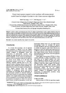
x ≥ cH ⎧1 ⎪ 2 ⎛ x − cL ⎞ ⎪ f ( x ) = ⎨ε + (1 − ε ) ⎜ (10) cL ≤ x < cH ⎟ ⎝ cH − cL ⎠ ⎪ ⎪ε x < cL ⎩ where cH , cL are two factors which are affected by the disperse degree of the data samples and can be got by typical experiment. ε is a lowest value which means the data is an outlier. Here these parameters are typically chosen as cH = 0.9, cL = 0.67, ε = 10−4 . ( xi , yi )

Di

Sik

Ri Oi

Fig. 1. Outlier Detected

As is shown in Fig. 1, the data point ( xi , yi ) , which is far away from the center of its neighborhood, is inclined to be an outlier and might be endowed with a lower memebership according to the heuristic function. 4. Simulation results

In this section, the proposed method is implemented and tested on two benchmark datasets: sinc function and Motorcycle datasets. The root mean square error (RMSE) is considered to verify the performance of the new method: 1 N 2 (11) RMSE = ∑ ( yi − yˆi ) N i =1 where N is the number of the data sample, yi and yˆi are real value and predicting value. The first benchmark datasets are generated by sinc function: sin x y= + ς , x ∈ [−10,10] (12) x where ς is a random noise such that ς = N ( 0, 0.04 ) . There are 125 data points produced by Eq.(12), 100 of which are randomly selected as training sets and the left are considered as test sets. In order to demonstrate the robust performance of our method, two artificial data points 4ς are added as outliers. The

1359 5

Lü Lü YouYou et al. Engineering 15 00 (2011) 1355 – 1360 ,et /alProcedia / Procedia Engineering (2011) 000–000

RMSE of training sets (RMSEtr) and test sets (RMSEte) are respectively illustrated in Tab.1. The setting σ and cost parameter c are got by grid search using 5-fold cross-validation. In order to compare the results conveniently, we call the classical LS-SVM without weight as LS-SVM and that with Suyken’s weight as WLS-SVM. The new method proposed in this paper is called as RLSSVM. Table 1. Comparison of LS-SVM, WLS-SVM and RLS-SVM

σ

c 39.42

3.27

RMSE

LS-SVM

WLS-SVM (13 times iteration)

RLS-SVM

RMSEtr

0.1450

0.0581

0.0301

RMSEte

0.1211

0.0612

0.0318

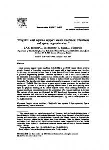
The fitting and predicting results are shown in Fig.2. The right figure is some enlarged parts of the left one. It is visable that the LS-SVM suffers more from outliers (denoted by ‘∗’) and RLS-SVM yields better performance. 3

sinc function training data

1.2 sinc function training data

test data

2

1

outlier

test data

LS-SVM RLS-SVM WLS-SVM

sinc(x)

sinc(x)

1

0

0.8

outlier

0.6

RLS-SVM WLS-SVM

LS-SVM

0.4 0.2

-1

0 -2

-3 -10

-0.2 -0.4 -8

-6

-4

-2

0 x

2

4

6

8

10

0.5

1

1.5

2

2.5

3

x

Fig. 2. Sinc Simulation: Comparison of LS-SVM, WLS-SVM and RLS-SVM

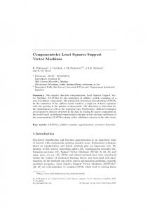
The next simulation is Motorcycle Dataset, a well-known benchmark dataset in the fields of statistics and robust regression. The tuning parameters are chosen according to [5]: σ = 6.6, c = 2 .The comparative results are shown in Fig.3. It is obvious that LS-SVM and WLS-SVM are more subjected to the boundary effects with oscillatory behavior (Time from 40 to 60) and RLS-SVM improves in this region. 100

training data test data LS-SVM RLS-SVM WLS-SVM

Head Acceleration

50

0

-50

outlier

-100

-150

0

10

20

30 Time

40

50

Fig. 3. Motorcycle Dataset Simulation: Comparison of LS-SVM, WLS-SVM and RLS-SVM

60

1360 6

/ Procedia Engineering (2011) 1355 – 1360 Lü Lü YouYou ,et et al/al. Procedia Engineering 00 15 (2011) 000–000

5. Conclusions In this study, a novel RLS-SVM is developed to deal with the training data sets containing outliers. Two benchmark data sets are simulated to verify the performance of the proposed approach. The regression results of the new method are much better than the weighted LS-SVM and classical LS-SVM. Besides, what is the most important is the fuzzy membership of each data point is assigned using a heuristic method instead of iterative training so that the computation complexity is reduced.

6. Acknowledgements This work has been supported by the National Natural Science Foundation of China (51036002/E060106): Basic Research on Energy Conservation and Optimization Control in Thermal Electricity System and the Joint Project of Beijing Education Committee.

References [1] V. Vapnik. The nature of statistical learning theory. New York: Springer, 1995. [2] V. Vapnik. Statistical learning theory. New York: Wiley, 1998. [3] J.A.K. Suykens, J. Vandewalle. Least squares support vector machine classiers. Neural Processing Letters, vol. 9, p. 293300, 1999. [4] S. Jooyong, H. Changha, N. Sunkyun. Robust LS-SVM regression using guzzy C-means clustering. Advances in Natural Computation, vol. 4221, p.157-166, 2006. [5] J.A.K. Suykens, J. De Brabanter, L. Lukas, J. Vandewalle. Weighted least squares support vector machines: robustness and sparse approximation. Neurocomputing, vol. 48, p. 85-105, 2002. [6] V. Cherkassky, Y. Ma. Practical selection of SVM parameters and noise estimation for SVM regression. Neural Networks, vol. 17, p.113-126, 2004. [7] Chuang Chen-Chia, et al.. Robust support vector regression networks for function approximation with outliers. IEEE Transaction on Neural Networks, vol. 13, p. 1322-1330, 2002. [8] Lin Chun-fu, Wang Sheng-de. Training algorithms for fuzzy support vector machines with noisy data. Pattern Recognition Letters, vol. 25, p. 1647-1656, 2004.