Broadcasting in Multi-Radio Multi-Channel Wireless Networks using ...

TECHNICAL REPORT TR-11-01, UC DAVIS, BBN, ARL, CUNY, PSU, JULY 2011.

1

Broadcasting in Multi-Radio Multi-Channel Wireless Networks using Simplicial Complexes W. Ren∗ , Q. Zhao∗ , R. Ramanathan†, J. Gao∗ , A. Swami‡ , A. BarNoy§ , M. Johnson¶ , P. Basu† ∗Department of Electrical and Computer Engineering, University of California, Davis, USA †Raytheon BBN Technologies, Cambridge, MA, USA ‡Army Research Laboratory, Adelphi, MD, USA §Department of Computer Science, City University of New York, USA ¶Department of Computer Science and Engineering, Pennsylvania State University, USA

Abstract We consider the broadcasting problem in multi-radio multi-channel ad hoc networks. The objective is to minimize the total cost of the network-wide broadcast, where the cost can be of any form that is summable over all the transmissions (e.g., the transmission and reception energy, the price for accessing a specific channel). Our technical approach is based on a simplicial complex model that allows us to capture the broadcast nature of the wireless medium and the heterogeneity across radios and channels. Specifically, we show that broadcasting in multi-radio multi-channel ad hoc networks can be formulated as a minimum spanning problem in simplicial complexes. We establish the NP-completeness of the minimum spanning problem and propose two approximation algorithms with order-optimal performance guarantee. The first approximation algorithm converts the minimum spanning problem in simplical complexes to a minimum connected set cover problem. The second algorithm converts it to a nodeweighted Steiner tree problem under the classic graph model. These two algorithms offer tradeoffs between performance and time-complexity. In a broader context, this work appears to be the first that studies the minimum spanning problem in simplicial complexes and weighted minimum connected set cover problem.

Index Terms 0

This work was supported by the Army Research Laboratory NS-CTA under Grant W911NF-09-2-0053.


2

Broadcast, multi-radio, multi-channel, ad hoc network, simplicial complex, minimum spanning, minimum connected set cover.

I. I NTRODUCTION Multi-Radio Multi-Channel (MR-MC) wireless networking arises in the context of wireless mesh networks, dynamic spectrum access via cognitive radio, and next-generation cellular networks [1, 2]. By the use of multiple channels, adjacent transmissions can be carried over non-overlapping channels to avoid mutual interference. Furthermore, each node, equipped with multiple radios, is capable of working in a full-duplex mode by tuning the transmitting and receiving radios to two non-overlapping channels. The increasing demand for high data rate and the persistent reduction in radio costs have greatly stimulated research on MR-MC networks. Considerable work has been done on capacity analysis [1], channel and radio assignment [3–8], and routing protocols [4, 5, 7, 9]. Considerable work has also been done on broadcasting in Single-Radio Single-Channel (SR-SC) networks [10– 13]. In this technical report, we consider the broadcasting problem in MR-MC ad hoc networks. A. Broadcasting in SR-SC Networks Broadcasting is a basic operation in wireless networks for disseminating a message containing, for example, situation awareness data and routing control information, to all nodes. For an SRSC network, a key question for the network-wide broadcast is which set of nodes should be selected to transmit during the broadcast such that the total cost is minimized. The cases where the cost is energy consumption [10, 11], the number of transmissions [12], or the overhead in route discovery and management [13] have been well studied. Recently, a unified solution to the minimum cost broadcasting problem, where the cost function can have various forms, has been proposed based on the formulation of the so-called neighborhood complex [14]. In contrast to their counterparts in wired networks which have polynomial solutions, the broadcast problems for minimizing the energy consumption and the number of transmissions are shown to be NP-complete in [11, 12]. The complexity of the broadcasting comes from the broadcast nature of the wireless medium: via an omnidirectional antenna, a single transmission from one node can reach all the other nodes


3

within the transmission range of this node, but it may cause interference to other nearby transmissions. This “node-centric” nature of the wireless broadcasting problem along with the mutual interference between concurrent transmissions complicates the design of efficient broadcasting algorithms. B. Broadcasting in MR-MC Networks In an MR-MC ad hoc network, such as the DARPA Wireless Network after Next (WNaN) [15], each node is equipped with multiple radios each operating on a different channel. The introduction of multiple channels and multiple radios further complicates the design of an efficient broadcasting scheme. Since the number of radios is usually smaller than the number of channels, the broadcast scheme should decide not only which nodes act as relays but also for those relay nodes, which channel(s) should be assigned to the transmitting radio(s). Given the selection of the relay nodes, two simple broadcast schemes [5] are: (i) transmitting multiple copies of the message on all channels; (ii) transmitting a single copy of the message on a common channel dedicated to broadcasting. Both schemes are inefficient. For the latter one, if the broadcast load is high, the common channel will be overwhelmed, even while there are plenty of other channels free. One subtle issue is the complication of the wireless broadcast advantage. In an MR-MC network, if the radios of the neighboring nodes are tuned to different channels, a single transmission on one channel cannot reach all the neighboring nodes simultaneously. In other words, only the neighboring nodes on the same channel can share the wireless broadcast advantage. More precisely, the concept of neighborhood must be defined both by radio range and channel. Another subtle issue is channel heterogeneity. Channels may have different bandwidth, fading condition, and accessing cost, leading to different implications in the total broadcast cost. Broadcasting in MR-MC networks is thus a multi-faceted problem, involving channel assignment, relay node selection, and channel selection for the source and relay nodes. In this technical report, we focus on the latter two issues by assuming a given channel-to-radio assignment. To avoid the hidden channel problem [8], two nodes that are two-hops away from each other are assigned two distinct sets of channels. Our design objective is to minimize the total broadcast cost, where the cost can be of any form that is summable over all the transmissions, including,


4

for example, the transmission and reception energy1 , the price for accessing each channel. C. A Simplicial Complex Model for Broadcasting in MR-MC Networks Our technical approach is based on a simplicial complex model of the broadcasting problem in MR-MC networks. A simplicial complex is a collection of nonempty sets with finite size that is closed under the subset operation. In other words, if a set s belongs to the collection, all subsets of s also belongs to the collection. An element of the collection is called a simplex or face. This constraint is often satisfied in the network context. For example, subsets of a broadcast/multicast group are broadcast/multicast groups, subsets of a clique are cliques. A simple example of graph and simplicial complex is given in Fig. 1. While the concept of simplicial complex has been around since the 1920’s, many well-solved fundamental problems in graph remain largely open under this more general model. v0

v1

v0

v2

v1

(a) Graph Fig. 1.

Graph and simplicial complex: V

v2

(b) Simplicial Complex =

{v0 , v1 , v2 }, S(a)

=

{(v0 , v1 ), (v0 , v2 ), (v1 , v2 )}, S(b)

=

{(v0 , v1 , v2 ), (v0 , v1 ), (v0 , v2 ), (v1 , v2 ), (v0 ), (v1 ), (v2 )}.

We use a simplicial complex model rather than a graph because the simplicial complex more naturally captures the broadcast channel, and the distinction and disjointness between broadcasting on different channels. Further, costs can be attached to faces (simplices) in a way not easily possible with graphs. 1

The ‘reception energy’ denotes the energy consumed by the radio in reception mode.


5

Consider an example MR-MC network. As shown in Fig. 2, after the channels are assigned, the network is partitioned into cliques of nodes. A clique consists of the nodes which share at least one common channel, and two cliques are spliced via nodes operating on multiple channels commonly shared by the two cliques. Within each clique, depending on the cost function, the transmitter decides which dimension simplex (i.e., a subclique or the clique itself) in a clique complex to activate. The message for the network-wide broadcast is thus propagated through a sequence of cliques, possibly of different dimensions. Note that the unicast case corresponds to a clique of dimension 1 (an edge). This example could also apply to the case where nodes may have multiple radios, perhaps of different modality (e.g., RF and optical); in this case, there may also be a cost associated with switching modes.

{f2 , f7 }

{f1 , f2 } {f4 , f6 }

{f3 , f8 }

{f1 , f3 }

{f1 , f4 , f5 }

{f5 , f6 }

Fig. 2. An illustration of an MR-MC network and the constructed simplicial complex. The parameters within the braces are the channels which each node can access. In the communication graph derived from the network, a link exists between two nodes if and only if two nodes are within each other’s transmission range and they share at least one common channel. Notice that a clique in the communication graph may not be a clique in the MR-MC network (correspondingly, a simplex in the simplicial complex), e.g., the three nodes of the right empty triangle.

In this case, the network-wide broadcast problem can be formulated as the minimum spanning problem in simplicial complexes. A clique in the MR-MC network is modeled as a simplex in the simplicial complex (see Fig. 2), and since a subset of a clique is still a clique, the constructed simplicial complex meets the requirement of being closed under the subset operation. The minimum spanning problem in a simplicial complex is to find a connected subset of simplices that covers all the vertices with the minimum total weight, i.e., the Minimum Connected


6

Spanning Subcomplex (MCSSub)2 . Then the solution to the network-wide broadcast problem can be obtained by solving the MCSSub problem. D. Minimum Spanning Problem in Simplicial Complexes The minimum spanning problem in a graph is to find a connected subgraph that covers all the vertices with minimum total weight. The solution must be a tree for graphs with nonnegative weights (hence called the Minimum Spanning Tree (MST)). There are several polynomial-time algorithms for MST, e.g., Kruskal’s Algorithm and Prim’s Algorithm [16]. The MST problem has many applications in network planning, broadcasting in communication networks, touring problems, and VLSI design [17]. With the addition of high dimensional simplices, the minimum spanning problem in a simplicial complex is fundamentally different and much more difficult than its counterpart in a graph. First, unlike the case in a graph, the MCSSub of a simplicial complex may not be a “tree”3 . As illustrated in Fig. 3, the MCSSub of the simplicial complex is the three filled triangles which form a cycle. Second, while simple greedy-type polynomial-time algorithms exist for finding the minimum spanning tree in a graph, the minimum spanning problem in a simplicial complex is NP-complete as established in this technical report (see Sec. III-A). We thus develop polynomial-time approximation algorithms for the minimum spanning problem in simplicial complexes. We propose two algorithms: one reduces this problem to a minimum connected set cover problem, and the other reduces the problem to a node-weighted Steiner tree problem in a graph derived from the original simplicial complex. We also establish the approximation ratios of the two algorithms. Both are shown to be order-optimal. The timecomplexity of these two algorithms is also analyzed, illustrating the tradeoff between performance and complexity offered by these two algorithms. In a broader context, this work appears to be the first that studies the minimum spanning problem in simplicial complexes and weighted minimum connected set cover problem. 2

Strictly speaking, a subcomplex should also be closed under the subset operation, but without loss of generality, we do

not include this condition in the definition of minimum connected spanning subcomplex, which is also more relevant to the broadcasting problem at hand. 3

Although there is no unified definition of tree in simplicial complexes, a couple of definitions can be obtained by generalizing

those equivalent definitions of tree in a graph. For example, simplicial trees can be defined based on the universal existence of leaves in any subgraph, or the uniqueness of simplicial facet paths.


7

v0 2

2 v1

v2 1

1 2

2

2

2

2

v3

v4

1 2

2 v5

Fig. 3.

A simplicial complex where its MCSSub is the three filled triangles, and is not a “tree” (the integers are the weights

of the simplices).

E. Related Work Broadcasting in MR-MC networks, mostly in the context of wireless mesh networks, has been studied for different optimization objectives [8, 18–23]. A channel assignment algorithm that minimizes interference among nodes in a multicast routing tree is proposed in [8]. Several heuristic algorithms for minimizing the broadcast latency are presented in [18, 19], where the broadcast latency is defined as the maximum delay between the transmission of a packet by the source node and its eventual reception by all the other nodes. Efficient broadcast algorithms are designed to minimize the total number of transmissions in [20] or the total number of radios used in the broadcast4 in [21]. In [18–21], the NP-hardness of the corresponding broadcast problems is established. The broadcast latency and the number of transmissions are minimized simultaneously in [22]. A widest spanning tree is constructed in [23] to maximize the bottleneck link bandwidth of the tree such that the content update time is minimized. 4

Notice that the total number of radios counts not only the transmitting radios but also the receiving radios, and thus it is

strictly greater than the total number of transmissions.


8

Different from the previous work, the optimization objective in our work can be any cost function which is summable over all the transmissions, thus taking into account channel heterogeneity (e.g., transmissions on different channels may consume different amounts of energy, due to different bandwidths or different propagation characteristics or some other factor). We point out that neither minimizing the total number of transmissions nor minimizing the total number of radios used in the broadcast is, in general, equivalent to minimizing the total energy consumption. The reception energy is ignored if the total number of transmissions is minimized, while the transmission energy and the reception energy are equated if the total number of radios is minimized. More importantly, channel heterogeneity is not addressed if these two objectives are optimized. Furthermore, to our best knowledge, our work is the first to adopt simplicial complexes to model and solve the broadcast problem in wireless ad hoc networks. An attempt to formulating the broadcast problem in wireless ad hoc networks into problems in simplicial complexes can be found in [14]. The simplicial complex is an important topic in algebraic topology. A detailed analysis based on homology and cohomology can be found in [24, 25]. Homology theory and techniques have been adopted as a computation tool for detecting and locating the coverage holes in sensor networks [26–28], and for deducing the topological information of the physical space from the encounter data of mobile networks [29]. Simplicial complexes can also be considered as special hypergraphs with the added constraint on the closedness under the subset operation. Here we adopt the simplicial complex model instead of the more general hypergraph model, because broadcasting does exhibit subset closure (i.e., one node can choose to broadcast to any subset of other nodes within the same clique). II. BASIC C ONCEPTS

IN

S IMPLICIAL C OMPLEXES

In this section, we introduce several basic concepts in simplicial complexes [24, 25]. An (abstract) simplicial complex is a collection ∆ of nonempty sets with finite size such that if A ∈ ∆, then ∀ B ⊆ A, B ∈ ∆, i.e., ∆ is closed under the operation of taking subsets. The element A of ∆ is called a simplex of ∆; its dimension (denoted by dim A) is one less than the number of its elements. Each nonempty subset of A is called a face of A. The dimension of ∆ is the maximum dimension over all its simplices, or is infinite if the maximum does not exist. The vertex set V of ∆ is the union of the one-point elements of ∆. Fig. 4 shows an example


9

of a 2-dimensional simplicial complex. A subcollection of ∆ that is itself a simplicial complex is called a subcomplex of ∆. A subcomplex of ∆ is the p-skeleton of ∆, denoted by ∆(p) , if it is the collection of all simplices of ∆ with dimension no larger than p. Thus, the 1-skeleton is the underlying graph of ∆. v5

v0

v1

v2

Fig. 4.

v3

v4

A simplicial complex ∆ with 6 vertices (0-dimensional simplices: {v0 },{v1 },{v2 },{v3 },{v4 },{v5 }), 5 edges (1-

dimensional simplices: {v1 , v2 },{v2 , v3 },{v3 , v4 },{v3 , v5 },{v4 , v5 }), and 1 filled triangle (2-dimensional simplex: {v3 , v4 , v5 }).

Any abstract simplicial complex has a geometric realization. There is a one-to-one correspondence between each element A = {v0 , ..., vn } of ∆ and a simplex spanned by the vertices v0 , ..., vn in Euclidean space. It can be shown that every d-dimensional simplicial complex can be realized in R2d+1 . Take graphs as a special example, which are 1-dimensional simplicial complexes: non-planar graphs cannot be embedded in R2 , but all the graphs can be realized in R3 . A facet of a simplicial complex ∆ is a maximal face of ∆, i.e., it is not a subset of any other face. A simplicial complex is connected if its 1-skeleton (i.e., the underlying graph) is connected in the graph sense. A weighted simplicial complex (WSC) ∆ is a triple (V, S, w)5 , where V is the set of vertices, S the set of faces of ∆, and w : S → {R+ ∪ {0}} a nonnegative weight function defined for each face in S with w(v) = 0 for all v ∈ V . We define the facet-only weight WF (∆) of a WSC 5

(S, w) suffices to denote the WSC since V ⊆ S, but we use the redundant (V, S, w) for convenience.


10

∆ as WF (∆) =

X

w(Fi ).

Fi ∈{facet of ∆}

III. M INIMUM C ONNECTED S PANNING S UBCOMPLEX In this section, we show that the MCSSub problem is NP-complete, and we propose two approximation algorithms based on connected set cover and node-weighted Steiner tree. We also establish the approximation ratios of the two algorithms and analyze their time complexity. A. NP-Completeness The decision version (D-MCSSub) of the MCSSub problem is stated as follows: let V (∆) denote the vertex set of a WSC ∆ and WF (∆) the facet-only weight of ∆. Given a WSC ∆ = (V, S, w) and K > 0, is there a connected subcomplex ∆sub of ∆ such that V (∆sub ) = V and WF (∆sub ) ≤ K? Then we have the following theorem. Theorem 1: The D-MCSSub problem is NP-complete. To prove the NP-completeness, we reduce the classic NP-complete problem – the unweighted set cover problem to the MCSSub problem. Proof: To check a solution to the D-MCSSub problem, we only need to verify the following points: (i) compute the facet-only weight of the solution and compare the weight with K; (ii) check whether the underlying graph of the solution is connected or not; (iii) check whether all the vertices of the original simplicial complex are covered by the solution. Since all these can be done within polynomial time, the D-MCSSub problem is NP. Given is an unweighted Set Cover instance I, i.e., a universe of elements U and a family of subsets F of U. For each element u ∈ U, we introduce a corresponding vertex in MCSSub instance I ′ . We introduce one additional vertex d. For each set f ∈ F , we introduce a corresponding face f ′ = f ∪ {d}, of weight 1. Being a simplcial complex, all subsets of f ′ are also introduced, all also of weight 1. In addition to covering all vertices, a solution to I ′ must be connected. Given any solution SOL to I of cost c, we can construct a solution to I ′ also of cost c. For every set f in SOL not including d, replace f with f ∪ {d}. On the other hand, given any solution SOL′ to I ′ of cost c, a solution to I of the same cost can be constructed as follows: for any face f ∈ SOL′ such that f does not appear as a set in


11

F , replace f with any superset of f − {d} appearing in F . Note that there must exist at least one such superset. This proof is for general D-MCSSub problems. It can be shown that even if the weight function of the WSC is monotone or strictly monotone6, the D-MCSSub problem is NP-hard. But it is still possible that the D-MCSSub problem under some special structured weight function is P. In the following, we present two approximation algorithms for the MCSSub problem both with performance guarantee O(ln n), where n is the number of vertices in the WSC. Since the best possible approximation ratio for the set cover problem is ln n [30], these two algorithms are order-optimal. B. Algorithm Based on Connected Set Cover Let A be a set with finite number of elements, and B = {Bi ⊆ A : i = 1, ..., n} a collection of subsets of A where each Bi is associated with a weight w(Bi ) ≥ 0. Let G be a connected graph with the vertex set B. A connected set cover (CSC) SC with respect to (A, B, w, G) is a set cover of A such that SC induces a connected subgraph of G. The minimum connected set cover (MCSC) problem is to find the CSC with the minimum weight, where the weight of a CSC SC is defined as w(SC ) =

X

w(Bi ).

Bi ∈SC

From a WSC ∆ = (V, S, w), we derive an auxiliary undirected graph G∆ in the following way: let S \ V be the vertex set of G∆ , and connect two vertices (non-vertex faces in ∆) S1 and S2 if and only if S1 ∩ S2 6= ∅. Then we have the following theorem on the relation between the MCSSub problem and the MCSC problem. Theorem 2: Let ∆∗ be the MCSSub of a WSC ∆ = (V, S, w) and SC∗ the MCSC of (V, S \ V, w, G∆ ). Then we have wF (∆∗ ) = w(SC∗ ). Proof: The proof is based on the following lemma. Lemma 1: Let SC∗ be the MCSC of (V, S \ V, w, G∆ ). For any face S ∈ SC∗ with w(S) > 0, we have that there does not exist a face S ′ ∈ SC∗ such that S ⊂ S ′ . 6

We say that the weight function satisfies the monotone property if for any two faces S1 ⊆ S2 , w(S1 ) ≤ w(S2 ), i.e., the

weight is monotone non-decreasing with respect to the dimension of the face.


12

Proof of Lemma 1: Suppose that for some face S ∈ SC∗ with w(S) > 0, ∃ S ′ ∈ SC∗ such that S ⊂ S ′ . Let SC′ = SC∗ \ s. Obviously, SC′ is a set cover, and w(SC′ ) = w(SC∗ ) − w(S) < w(SC∗ ). On the other hand, since S ∩ S ′′ 6= ∅ implies S ′ ∩ S ′′ 6= ∅ for any face S ′′ ∈ SC∗ , it follows from the connection rule of the auxiliary graph G∆ that any path via S has an alternative path via S ′ . Thus, SC′ is a CSC, leading to a contradiction. Given the MCSC SC∗ of (V, S \ V, w, G∆ ), we can obtain a connected spanning subcomplex ∆∗C by mapping each element of SC∗ to a face in ∆. Since the facet-only weight wF (∆∗C ) of ∆∗C only counts facets in ∆∗C , it follows that wF (∆∗C ) ≤ w(SC∗ ). Based on Lemma 1, we have that every element of SC∗ with positive weight is a facet in ∆∗C , and thus wF (∆∗ ) ≤ wF (∆∗C ) = w(SC∗ ), where ∆∗ is the MCSSub of ∆. ∗ ∗ On the other hand, the facets of ∆∗ leads to an CSC S∆ , and w(S∆ ) = wF (∆∗ ). It implies

that ∗ w(SC∗ ) ≤ w(S∆ ) = wF (∆∗ ).

Thus, wF (∆∗ ) = w(SC∗ ). 1) Algorithm: Based on Theorem 2, we can reduce the MCSSub problem of a WSC ∆ = (V, S, w) to the MCSC problem (V, S \ V, w, G∆ ). We obtain the following Set Cover based Algorithm (SCA) for the MCSSub problem.

Algorithm 1: SCA for MCSSub: INPUT: A WSC ∆ = (V, S, w). OUTPUT: An approximate MCSSub ∆C of ∆. 1. Derive the auxiliary graph G∆ . 2. Find an approximate MCSC SC of (V, S \ V, w, G∆ ) by using the greedy algorithm for MCSC (Algorithm 2). 3. Transform SC to a connected spanning subcomplex ∆C by mapping each element of SC to a face in ∆.


13

Zhang et al. propose a greedy approximation algorithm for the unweighted MCSC problem [31]7 , i.e., w(Bi ) = 1 for all i. By generalizing their greedy approach, we develop a greedy algorithm for the weighted MCSC problem. Before stating the algorithm, we introduce the following notations and definitions. For two sets S1 , S2 ∈ S, let distG (S1 , S2 ) be the length of the shortest path between S1 and S2 in an auxiliary graph G, where the length of a path is given by the number of edges; S1 and S2 are said to be graph-adjacent if they are connected via an edge in G (i .e., distG (S1 , S2 ) = 1), and they are said to be cover-adjacent if S1 ∩ S2 6= ∅. Notice that in a general MCSC problem, there is no connection between these two types of adjacency. The cover-diameter DC (G) is defined as the maximum distance between any two cover-adjacent sets, i.e., DC (G) = max{distG (S1 , S2 ) | S1 , S2 ∈ S and S1 ∩ S2 6= ∅}. For the MCSC problem derived from the MCSSub problem of a WSC ∆, we have that DC (G∆ ) = 1. At each step of the algorithm, let R denote the collection of the subsets (faces of ∆) that have been selected, and U the vertex subset of ∆ that has been covered. Given R = 6 ∅ and a set S ∈ S \ R, an R → S path is a path {S0 , S1 , ..., Sk } in G such that (i) S0 ∈ R; (ii) Sk = S; (iii) S1 , ..., Sk ∈ S \ R. We define the weight ratio r(PS ) of PS as P w(S(PS ) \ R) S∈S(PS )\R w(S) = , r(PS ) = |VN (PS )| |VN (PS )|

(1)

where S(PS ) \ R is the subsets (faces in S) of PS that are not in R, and |VN (PS )| is the number of vertices of ∆ that are covered by PS but not covered by R. Algorithm 2: A Greedy Algorithm for MCSC. INPUT: (V, S \ V, w, G∆ ) OUTPUT: A CSC R. 1. Choose S0 ∈ S \ V such that the weight ratio r(S0 ) defined in (1) is the minimum, and let R = {S0 } and U = S0 . 2. WHILE V \ U 6= ∅ DO 7

The original algorithm in [31] has a flaw and the established approximation ratio is incorrect. In [32], the flaw is corrected

and a stronger result on the approximation ratio is shown.


14

2.1. For each S ∈ S \ (V ∪ R) which is cover-adjacent or graph-adjacent with a set in R, find a shortest8 R → S path PS . 2.2. Select PS with the minimum weight ratio r(PS ) defined in (1), and let R = R ∪ PS (add all the subsets of PS to R) and U = U ∪ VN (PS ). END WHILE 3. RETURN R.

2) Approximation Ratio: The approximation ratio of SCA is determined by Step 2, i.e., the approximation ratio of the greedy algorithm for the MCSC problem. First, we show the following lemma. Lemma 2: Given a weighted MCSC problem (V, S \ V, w, G) with DC (G) = 1, let max{w(S)} Rw =

S∈S

min{w(S)}

.

(2)

S∈S

Then the approximation ratio of the greedy algorithm for MCSC is at most Rw + H(γ − 1), where γ = max{|S| | S ∈ S \ V } is the maximum size of the subsets in S and H(·) is the harmonic function. Proof of Lemma 2: The proof is based on the classic charge argument. Let S ∗ be an optimal solution to the weighted set cover problem (V, S \ V, w), and R the solution returned by the greedy algorithm for the weighted MCSC problem (V, S \ V, w, G) with DC (G) = 1. Let w(S ∗ ) and w(R) denote the total weight of the subsets included in S ∗ and R, respectively. In the following, we will show that w(R) ≤ Rw + H(γ − 1). w(S ∗ )

(3)

Let SC∗ be an optimal solution to the weighted MCSC problem (V, S \ V, w, G) with DC (G) = 1. Since w(S ∗ ) ≤ w(SC∗ ), Lemma 2 follows immediately. To prove (3), we apply the classic charge argument. Each time a subset S0 (at step 1) or a shortest R → S path PS∗ (at step 2) is selected to be added to R, we charge each of the newly covered elements 8

w(S0 ) |S0 |

(at step 1) or r(PS∗) defined in (1) (at step 2). Notice that when

Notice that the shortest path is defined in terms of the number of edges, not the total weight of all vertices along the path.


15

DC (G) = 1, the shortest R → S path PS∗ is only a single edge connecting some subset in R and S, and r(PS∗) =

w(S(PS∗ \ R)) w(S) = . ∗ |VN (PS )| |S \ U|

During the whole procedure, each element of V is charged exactly once. Assume that step 2 ∗ is completed in K − 1 iterations. Let PSi be the shortest R → S path selected by the algorithm

at iteration i. Let C(v) denote the charge of an element v in V . Then we have that X

C(v) =

K−1 X

X

C(v)

∗ ) i=0 v∈VN (PSi

v∈V

=

K−1 X

X

i=0 v∈Si \U

=

K−1 X

w(Si ) |Si \ U|

w(Si ) = w(R),

(4)

i=0

where

∗ PS0

= {S0 }.

∗ Suppose that S ∗ = {S1∗ , ..., SN } is a minimum weighted set cover for {V, S \ V, w}. Since an

element of V may be contained in more than one subset of S ∗ , it follows that X

C(v) ≤

N X X

C(v).

(5)

i=1 v∈Si∗

v∈V

Next we will show an inequality which bounds from above the total charge of a subset in S ∗ , i.e., for any B ∗ ∈ S ∗ , X

C(v) ≤ [Rw + H(|S ∗| − 1)]w(S ∗).

(6)

v∈B ∗

Let ni (i = 0, 1, ..., K) be the number of elements of S ∗ that have not been covered by S after iteration i − 1, where step 1 is considered as iteration 0. Let {i1 , ..., ik } denote the subsequence of {i = 0, 1, ..., K − 1} such that ni − ni+1 > 0. For each element a covered at iteration i1 , if i1 = 0, based on the greedy rule at step 1, we have that w(S ∗ ) ; ≤ ni1

(7)

w(S ∗)Rw w(Si1 ) . ≤ |Si1 \ U| ni1 − n(i1 +1)

(8)

C(v) =

r(PS∗0 )

Otherwise, C(v) = r(PS∗i ) = 1


16

The inequality in (8) is due to the fact that Si1 covers at least ni1 − n(i1 +1) elements of V , i.e., |Si1 \ U| ≥ ni1 − n(i1 +1) . Summing up (7) and (8), C(v) ≤

w(S ∗ )Rw . ni1 − n(i1 +1)

(9)

Consider two cases: (i) If all the elements of S ∗ have been covered after iteration i1 , i.e., n(i1 +1) = 0, then X w(S ∗ )Rw X C(v) ≤ = w(S ∗)Rw . n 0 v∈S ∗ v∈S ∗

(10)

(ii) If not all the elements of S ∗ have been covered by R after iteration i1 , S ∗ becomes coveradjacent with R and thus a candidate for being selected at the following iterations. At each iteration, for each element v ∈ S ∗ covered at iteration ij (j = 2, ..., k), the greedy rule at step 2 still yields C(v) = r(PS∗i ) ≤ r(PS∗∗ ) j

w(S ∗ ) w(S ∗ ) . = |S ∗ \ U| nij

= It follows from (9,11) that X

C(v) ≤ (ni1 − n(i1 +1) )

v∈S ∗

+

k X

=

1 ni1 − n(i1 +1)

(nij − n(ij +1) )

j=2

(11)

1 nij !

k X nij − ni(j+1) 1+ nij j=2

.

(12)

Here we have used the fact that n(ij +1) = ni(j+1) . It is because between iteration ij and iteration i(j+1) , no elements of S ∗ are covered. For the summation term in (12), we have the following inequality: k X nij − ni(j+1) nij j=2

k X 1 1 ≤ +···+ n ni(j+1) + 1 j=2 ij

= H(ni2 ) ≤ H(|S ∗| − 1).

The last inequality is due to the fact that ni2 ≤ ni1 − 1 = |S ∗ | − 1.

(13)


17

Eqn. (6) is a direct consequence of (10), (12), and (13). Thus, using (4-6), N X X X C(v) w(R) = C(v) ≤ i=1 v∈Si∗

v∈V

≤

N X

[Rw + H(|Si∗| − 1)]w(Si∗)

i=1

≤ [Rw + H(γ − 1)]w(S ∗ ).

Then, as a direct consequence of Lemma 2, we have the following theorem on the approximation ratio9 of the greedy algorithm for the MCSC problem with DC (G) = 1. Theorem 3: Let ∆∗ be the MCSSub of a WSC ∆ = (V, S, w) and ∆C be the solution returned by Algorithm 1. Let Rw be defined as in (2). Then we have wF (∆C ) ≤ Rw + H(dim∆), wF (∆∗ ) where dim∆ is the dimension of ∆ and H(·) is the harmonic function. From Theorem 3, we see that the approximation ratio depends on the ratio Rw of the maximum weight to the minimum weight. It is shown in the following theorem that if Rw is unbounded, then the scaling order of the approximation ratio can be as bad as linear with respect to the number of vertices in the simplicial complex. Theorem 4: Let n be the number of the vertices in a WSC ∆ = (V, S, w), and Rw defined as in (2). If Rw is unbounded, then the approximation ratio of Algorithm 1 for the MCSSub problem of ∆ is Ω(n). Proof: Consider a specific example: ∆ is a (n − 1)-dimensional simplex with the vertex set V = {v1 , ..., vn }, and all the weights of the faces are infinite except for the following five faces: 1 = , w(S1 ) = w v1 , ..., v n2 2 n o 1 n w(S2 ) = w v1 , ..., v 4 , v( n +2) = , 2 2 o 1 n = , w(S3 ) = w v( n +1) , ..., v( n +1) 4 2 2 n w(S4 ) = w v n2 , ..., vn = , 8 n o w(S5 ) = w

9

v( n +1) , ..., vn 2

= 1.

The approximation ratio of the greedy algorithm for general weighted MCSC problem is still an open problem.


18

For ease of presentation, we have assumed that n is a multiple of 4. By applying Algorithm 1, we reduce the MCSSub problem for ∆ to the MCSC problem (V, S \ V, w, G∆ ). Due to the weight assignment, it suffices to only consider the subgraph of G∆ induced by the above five faces, as shown in Fig 5. S1 v1 , ..., v n2

S2

S3

S4

o n v1 , ..., v n4 , v( n +2) 2

v n2 , ..., vn

n

v( n +1) , ..., v( n +1) 4 2

S5 n o v( n +1) , ..., vn 2

Fig. 5.

The subgraph of G∆ induced by the five faces S1 , S2 , S3 , S4 , and S5 with finite weights.

The optimal solution ∆∗ to the MCSSub problem is given by ∆∗ = {S ∈ S | S ⊆ S2 or S3 or S5 }, and wF (∆∗ ) = w(S2 ) + w(S3) + w(S5) = 2. On the other hand, the solution ∆C returned by Algorithm 1 is given by ∆C = {S ∈ S | S ⊆ S1 or S4 }, and wF (∆C ) = w(S1 ) + w(S4 ) =

1 n + . 2 8

o


19

Specifically, S1 is firstly selected, and then S4 . Thus, n 1 wF (∆C ) = + = Θ(n). ∗ wF (∆ ) 16 4 It follows that the approximation ratio of Algorithm 1 is Ω(n). From Theorem 4, we see that Algorithm 1 is not suitable for the MCSSub problem of a WSC ∆ if its weight function has a relatively wide range. As shown next in Sec. III-C, the other approximation algorithm based on the Steiner tree does not have this issue: its approximation ratio does not depend on the range of the weight function. C. Algorithm Based on Steiner Tree From a WSC ∆ = (V, S, w), we derive an undirected graph H∆ with the vertex set S: for each face S ∈ S \ V (i.e., the faces that are not the vertices of ∆), we replace it by a vertex vS in H∆ and connect vS to all the vertices of S. The weight w(vS ) assigned to the vertex vS is the weight w(S) of the face S. Notice that the weight of vertices in H∆ corresponding to the vertices in ∆ (i.e., V) is zero. Fig. 6 shows an example of the derivation of the graph from a 2-simplex. We have the following theorem on the relation between the MCSSub of ∆ and the Steiner tree of H∆ that spans the vertex set V of ∆ and the minimum connected dominating set10 of H∆ . Theorem 5: Let ∆∗ denote the MCSSub of a WSC ∆ = (V, S, w), T ∗ the Steiner tree of H∆ that spans the vertex set V of ∆, and DC∗ the minimum connected dominating set of H∆ . Then we have that wF (∆∗ ) = w(T ∗ ) = w(DC∗ ). Proof: First we show that wF (∆∗ ) = w(T ∗ ). Since every connected spanning subcomplex ∆′ of ∆ corresponds to a connected subgraph of H∆ which only contains the vertices of ∆ and the vertices representing the facets of ∆′ , it follows that w(T ∗ ) ≤ wF (∆∗ ). On the other hand, since by contradiction, there is a one-to-one mapping between the vertices of the Steiner tree of 10

A dominating set of a graph is a subset of vertices such that every vertex of the graph is either in the subset or a neighbor

of some vertex in the subset, and a connected dominating set (CDS) is a dominating set where the subgraph induced by the vertices in the dominating set is connected. The CDS problem asks for a CDS with the minimum total weight, and it is shown to be a special case of the MCSC problem [32].


∆ Fig. 6.

20

H∆

The derived graph of a 2-simplex (squares in H∆ represent the faces that are not vertices of ∆).

H∆ and the vertices plus the facets of a connected spanning subcomplex of ∆, it follows that wF (∆∗ ) ≤ w(T ∗). Next we show that w(T ∗ ) = w(DC∗ ). Notice that the vertex set V of ∆ is a dominating set of H∆ . Since the Steiner tree T ∗ of H∆ spans the vertex set V , T ∗ is a CDS of H∆ . Thus, w(DC∗ ) ≤ w(T ∗ ). On the other hand, given the minimum CDS DC∗ of H∆ , since each vertex v in the vertex set V is either in DC∗ or a neighbor of some face in DC∗ and the weights of the vertices in V are all zero, the combination of V and DC∗ yields a connected subgraph of H∆ that spans V with the same weight as DC∗ . Thus, w(T ∗ ) ≤ w(DC∗ ). Based on Theorem 5, we propose the following Steiner Tree based Algorithm (STA) for the MCSSub problem.

Algorithm 3: STA for MCSSub: INPUT: A WSC ∆ = (V, S, w). OUTPUT: An approximate MCSSub ∆C of ∆. 1. Derive the graph H∆ from ∆. 2. Obtain an approximate Steiner tree T of H∆ by using the algorithms given in [33, 34]. 3. Transform T to a connected spanning subcomplex ∆C of ∆ by mapping each element of T to a face of ∆.


21

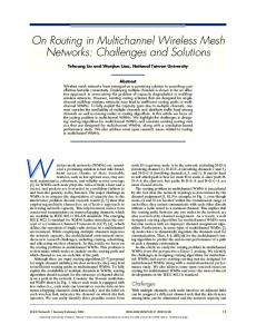
Since approximation only occurs in Step 2, the approximation ratio of STA is equal to that of the algorithm for the node-weighted Steiner tree problem. The best approximation ratio is known to be (1.35 + ǫ) ln n for any constant ǫ > 0, where n is the number of vertices of ∆ and is also the number of terminals in the Steiner tree of H∆ [34]. Here we do not try to find the CDS DC∗ of H∆ at step 2, because the best known approximation ratio for the CDS problem is (1.35 + ǫ) ln n(H∆ ) [34, 35]. Since n(H∆ ) ≫ n, the latter approximation ratio is much worse than the former one. D. Time Complexity Analysis Here we analyze the time complexity of SCA and STA for the MCSSub problem. Given a WSC ∆ = (V, S, w), let n = |V | denote the number of vertices in ∆, m = |S \ V | the number of non-vertex faces in ∆, and d the dimension of ∆. Recall that the existence of edges in the auxiliary graph G∆ for SCA and the derived graph H∆ for STA depends entirely on whether the two non-vertex faces overlap and whether the vertex is contained in the non-vertex face, respectively. It implies that all the information of these two graphs can be easily retrieved from the WSC ∆. Thus, Step 1 in both algorithms can be skipped in the implementation, and the time complexity of both algorithms is determined by their Step 2. Step 2 of SCA is to apply the greedy algorithm to the MCSC problem (V, S \ V, w, G∆ ). It takes O(m) time to complete Step 1 of the greedy algorithm. Since at least one vertex becomes covered at each iteration of Step 2 of the greedy algorithm, there are at most n − 1 iterations. At each iteration, the weight ratios of at most m faces are computed, and due to the fact that cover-adjacent faces are graph-adjacent, the weight ratio of each face is done in constant time. Thus, the running time of SCA is O(m + nm) = O(nm). Since the derived graph H∆ has n + m vertices and O(dm) edges and the Steiner tree has n terminals to cover, it follows from [36] that the running time of Step 2 of STA is O(dnm2 + nm2 log m). From the above, we see that the time complexity of STA is significantly higher than that of SCA. This is mostly because the approximation algorithm for the Steiner tree requires the computation of the shortest paths between all vertex pairs. We point out that while the Steiner tree based algorithm has a higher complexity, it can offer better performance in a WSC with a large weight range. In a simulation example of random simple complexes, we consider a case where each face weight takes only two values wmin and


22

wmax with equal probability. With wmin = 1, wmax = 10000, and 1000 Monte Carlo runs for a 200-vertex random simplicial complex11 [38], we find that the total weight of the solution returned by the set cover based algorithm can be 1.7 times that of the solution returned by the Steiner tree based algorithm. These two algorithms thus offer a tradeoff between performance and complexity. IV. S IMULATION R ESULTS In this section, we present simulation results on the performance of the two approximation algorithms (SCA and STA) for the broadcast problem in an MR-MC network. We consider a dense MR-MC network, where all the nodes are within each other’s transmission range, and we aim to minimize the total energy consumption of the broadcast. There are 12 non-overlapping channels fi (1 ≤ i ≤ 12), possibly with different communication rates ri , available for the MR-MC network, and each node is equipped with 4 radios. At the beginning of the broadcast, each node randomly selects 4 of the 12 channels for its 4 radios. As discussed in Sec. I-C, the nodes which share at least one common channel form a clique, and there is a one-to-one correspondence between the cliques and the faces of the derived WSC. The weight of the face is defined as the energy consumption of the broadcast within the corresponding clique, i.e., the sum of the transmission energy and the reception energy. Let S be a face containing k + 1 nodes and {fSj : j = 1, 2, ..., q} the q (1 ≤ q ≤ 12) common channels shared by the k + 1 nodes. Assume that if a node in the clique is selected as relay, it will choose the common channel with the maximum communication rate to transmit. Then the weight w(S) of the face S is given by w(S) = (Ptx + kPrx )

L , max {rSj }

j=1,...,q

where Ptx and Prx are the transmission power and the reception power, respectively, and L is a constant. 11

A random simplicial complex ∆(n, D, p ~) with n vertices, dimension at most D, and a D-dimensional probability vector

p ~ = {p1 , p2 , ..., pD } is constructed in a bottom-up manner: first n vertices are fixed, which are the 0-simplices of ∆, and then higher-dimensional simplices are generated inductively. Specifically, for each 1 ≤ i ≤ D, after all the simplices with dimension lower than i have been generated, consider every i-tuple of vertices: if they have formed all the lower dimensional simplices, then an i-simplex consisting of them is generated with probability pi . Notice that a random simplicial complex ∆(n, 1, p) is the random graph introduced by Erd˝os and R´enyi [37].


23

1000 900

SCA STA MST

Average Total Energy

800 700 600 500 400 300 200 100 0 20

Fig. 7.

30

40

50 60 Number of Nodes

70

80

90

Average total energy vs. number of nodes. Parameters: Ptx =1, Prx = 0.01, L = 100, ri = i for 1 ≤ i ≤ 12.

In Fig. 7, the average total energy of the solutions returned by SCA and STA is compared with that of the MST with respect to the underlying graph of the WSC. The average is taken over 10 random channel assignments. Notice that although two different links on the same channel are treated separately when the MST is derived, the transmission energy corresponding to them is counted only once to exploit the wireless broadcast advantage when the total energy of the MST is computed. We see that the performances of SCA and STA are extremely close, and their performances are significantly better than that of MST. V. C ONCLUSION

AND

F UTURE WORK

In this technical report, we study the minimum cost broadcast problem in multi-radio multichannel ad hoc networks, where the total cost is the sum of the costs associated with the transmissions during the broadcast. We formulate it into a fundamental problem, the minimum spanning problem, in simplicial complexes. Due to the existence of the simplices with dimension higher than edges, this minimum spanning problem is more complex than its counterpart in a ‘conventional’ graph for which simple polynomial algorithms exist. Specifically, it is shown to be NP-complete via a reduction from the set cover problem. We thus propose two approximation


24

algorithms for this minimum spanning problem: one is to transform it into the connected set cover problem; the other is to transform it into the node-weighted Steiner tree problem and then apply the corresponding algorithm. Despite their distinct approaches, the performance of both approximation algorithms is shown to be order-optimal. Furthermore, we show that there is a tradeoff in terms of performance vs. complexity: although the one based on connected set cover has lower time complexity than the one based on the Steiner tree, the performance of the former is sensitive to the weight range. As a starting point, we have assumed that the channel assignment scheme is designed independent of the broadcast scheme. The joint optimization of the two schemes will further reduce the broadcast cost. Another future direction is to develop distributed versions of the approximation algorithms for the minimum cost broadcast problem. R EFERENCES [1] P. Kyasanur and N. H. Vaidya, “Capacity of multi-channel wireless networks: Impact of number of channels and interfaces,” in Proc. of ACM MobiCom, August 2005, pp. 43–57. [2] P. Kyasanur, J. So, C. Chereddi, and N. H. Vaidya, “Multichannel mesh networks: Challenges and protocols,” IEEE Wireless Communications, vol. 13, no. 2, pp. 30–36, April 2006. [3] N. Jain, S. R. Das, and A. Nasipuri, “A multichannel csma mac protocol with receiver-based channel selection for multihop wireless networks,” in Proc. of ICCCN, October 2001, pp. 432–439. [4] A. Raniwala and T. Chiueh, “Architecture and algorithms for an ieee 802.11-based multi-channel wireless mesh network,” in Proc. of IEEE INFOCOM, March 2005, pp. 2223–2234. [5] P. Kyasanur and N. H. Vaidya, “Routing and interface assignment in multi-channel multi-interface wireless networks,” in Proc. of IEEE WCNC, March 2005, pp. 2051–2056. [6] J. Tang, G. Xue, and W. Zhang, “Interference-aware topology control and qos routing in multi-channel wireless mesh networks,” in Proc. of ACM MobiHoc, May 2005, pp. 68–77. [7] P. Kyasanur and N. H. Vaidya, “Routing and link-layer protocols for multi-channel multi-interface ad hoc wireless networks,” ACM SIGMOBILE Mobile Computing and Communications Review, vol. 10, no. 1, pp. 31–43, January 2006. [8] H. L. Nguyen and U. T. Nguyen, “Channel assignment for multicast in multi-channel multi-radio wireless mesh networks,” Wireless Communications and Mobile Computing, vol. 9, no. 4, pp. 557–571, April 2009. [9] V. Raman and N. H. Vaidya, “Short: A static-hybrid approach for routing real time applications over multichannel, multihop wireless networks,” Lecture Notes in Computer Science: Wired/Wireless Internet Communications, vol. 6074, pp. 77–94, 2010.


25

[10] J. E. Wieselthier, G. D. Nguyen, and A. Ephremides, “On the construction of energy-efficient broadcast and multicast trees in wireless networks,” in Proc. of IEEE INFOCOM, March 2000, pp. 585–594. ˇ [11] M. Cagalj, J. Hubaux, and C. Enz, “Minimum-energy broadcast in all-wireless networks: Np-completeness and distribution issues,” in Proc. of ACM MobiCom, September 2002, pp. 172–182. [12] W. Lou and J. Wu, “On reducing broadcast redundancy in ad hoc wireless networks,” IEEE Transactions on Mobile Computing, vol. 1, no. 2, pp. 111–122, April-June 2002. [13] C. Gui and P. Mohapatra, “Scalable multicasting in mobile ad hoc networks,” in Proc. of IEEE INFOCOM, March 2004, pp. 2119–2129. [14] R. Ramanathan, A. Bar-Noy, P. Basu, M. Johnson, W. Ren, A. Swami, and Q. Zhao, “Beyond graphs: Capturing groups in networks,” IEEE NetSciCom (to appear), April 2011. [15] M. Lawlor, “Wireless to the nth degree,” AFCEA Signal Online, July 2006. [Online]. Available: http://www.afcea.org/signal/articles/templates/SIGNAL Article Template.asp?articleid=1150&zoneid=188 [16] J. Kleinberg and E. Tardos, Algorithm Design. Boston, MA: Addison Wesley, 2005. [17] C. F. Bazlamacci and K. S. Hindi, “Minimum-weight spanning tree algorithms: A survey and empirical study,” Computers & Operations Research, vol. 28, no. 8, pp. 767–785, July 2001. [18] C. T. Chou, A. Misra, and J. Qadir, “Low-latency broadcast in multirate wireless mesh networks,” IEEE Journal on Selected Areas in Communications (JSAC), vol. 24, no. 11, pp. 2081–2091, November 2006. [19] J. Qadir, A. Misra, and C. T. Chou, “Minimum latency broadcasting in multi-radio multi-channel multi-rate wireless meshes,” in Proc. of IEEE SECON, September 2006, pp. 80–89. [20] L. Li, B. Qin, C. Zhang, and H. Li, “Efficient broadcasting in multi-radio multi-channel and multi-hop wireless networks based on self-pruning,” in Proc. of HPCC, September 2007, pp. 484–495. [21] K. Han, Y. Li, Q. Guo, and M. Xiao, “Broadcast routing and channel selection in multi-radio wireless mesh networks,” in Proc. of IEEE WCNC, March 2008, pp. 2188–2193. [22] M. Song, J. Wang, and Q. Hao, “Broadcasting protocols for multi-radio multi-channel and multi-rate mesh networks,” in Proc. of IEEE ICC, June 2007, pp. 3604–3609. [23] H. S. Chiu, B. Wu, K. L. Yeung, and K. S. Lui, “Widest spanning tree for multi-channel multi-interface wireless mesh networks,” in Proc. of IEEE WCNC, March 2008, pp. 2194–2199. [24] J. R. Munkres, Elements of Algebraic Topology. Menlo Park, CA: Addison-Wesley, 1984. [25] A. Hatcher, Algebraic Topology. New York: Cambridge University Press, 2002. [26] R. Ghrist and A. Muhammad, “Coverage and hole-detection in sensor networks via homology,” in Proc. of IPSN, April 2005, pp. 254–260. [27] J. Derenick, V. Kumar, and A. Jadbabaie, “Towards simplicial coverage repair for mobile robot teams,” in Proc. of IEEE ICRA, May 2010, pp. 5472–5477. [28] H. Chintakunta and H. Krim, “Divide and conquer: Localizing coverage holes in sensor networks,” in Proc.


26

of IEEE SECON, June 2010, pp. 359–366. [29] B. D. Walker, “Using persistent homology to recover spatial information from encounter traces,” in Proc. of ACM MobiHoc, May 2008, pp. 371–380. [30] U. Feige, “A threshold of ln n for approximating set cover,” Journal of the ACM, vol. 45, no. 4, pp. 634–652, July 1998. [31] Z. Zhang, X. F. Gao, and W. L. Wu, “Algorithms for connected set cover problem and fault-tolerant connected set cover problem,” Theoretical Computer Science, vol. 410, no. 8-10, pp. 812–817, March 2009. [32] W. Ren and Q. Zhao, “A note on: ‘algorithms for connected set cover problem and fault-tolerant connected set cover problem’,” Submitted to Theoretical Computer Science, February 2011. [Online]. Available: http://arxiv.org/abs/1104.0733 [33] P. N. Klein and R. Ravi, “A nearly best-possible approximation algorithm for node-weighted steiner trees,” Journal of Algorithms, vol. 19, no. 1, pp. 104–115, July 1995. [34] S. Guha and S. Khuller, “Improved methods for approximating node weighted steiner trees and connected dominating sets,” Information and Computation, vol. 150, no. 1, pp. 57–74, April 1999. [35] ——, “Approximation algorithms for connected dominating sets,” Algorithmica, vol. 20, no. 4, pp. 374–387, April 1998. [36] W. F. Liang, “Approximate minimum-energy multicasting in wireless ad hoc networks,” IEEE Transactions on Mobile Computing, vol. 5, no. 4, pp. 377–387, April 2006. [37] P. Erd˝os and A. R´enyi, “On the evolution of random graphs,” in Publication of the Mathematical Institute of the Hungarian Academy of Sciences, 1960, pp. 17–61. [38] M. A. Mannucci, L. Sparks, and D. C. Struppa, “Simplicial models of social aggregation i,” April 2006. [Online]. Available: http://arxiv.org/abs/cs/0604090

Broadcasting in Multi-Radio Multi-Channel Wireless Networks using ...

Broadcasting in Multi-Radio Multi-Channel Wireless Networks using ...

Suggest Documents

Minimum Latency Broadcasting in Multiradio ... - Google Sites

Predictive Segmentation Using Multichannel Neural Networks in ...

Multichannel MAC Protocols for Wireless Networks - CiteSeerX

On Routing in Multichannel Wireless Mesh Networks: Challenges and ...

Improved Self-Pruning for Broadcasting in Ad Hoc Wireless Networks

Localized Techniques for Broadcasting in Wireless Sensor Networks

Deadline-aware Broadcasting in Wireless Networks with Local ...

Energy-aware Broadcasting in Wireless Networks - HAL-Inria

Maximum Lifetime Broadcasting In Wireless Networks - UF CISE

An Efficient Multichannel Wireless Sensor Networks MAC Protocol ...

Performance of multichannel wireless ad hoc networks ... - CiteSeerX

An Efficient Multichannel Wireless Sensor Networks MAC ... - Core

A Multichannel CSMA MAC Protocol for Multihop Wireless Networks ...

System Design Options for Video Broadcasting over Wireless Networks

Synchronization in Wireless Sensors Networks Using ...

Capacity Enhancement in Wireless Networks using ... - CiteSeerX

data gathering in wireless sensor networks using

NetDetect: Neighborhood Discovery in Wireless Networks Using ...

Performance improvement in wireless networks using ... - CiteSeerX

Localized Broadcasting in Mobile Ad Hoc Networks Using Neighbor ...

Cooperation diversity in multihop wireless networks using

Traffic improvements in wireless communication networks using

Ambisonics in Multichannel Broadcasting and Video - Google Sites

Localization Using Neural Networks in Wireless Sensor Networks