periments in this paper indicate neural networks are a vi- able option for solving ... We will introduce the use of a Radial Basis Function. (RBF) neural network for ...
Localization Using Neural Networks in Wireless Sensor Networks Ali Shareef, Yifeng Zhu∗ , and Mohamad Musavi Department of Electrical and Computer Engineering University of Maine Email: {ashareef, zhu∗ , musavi}@eece.maine.edu ABSTRACT Noisy distance measurements are a pervasive problem in localization in wireless sensor networks. Neural networks are not commonly used in localization, however, our experiments in this paper indicate neural networks are a viable option for solving localization problems. In this paper we qualitatively compare the performance of three different families of neural networks: Multi-Layer Perceptron (MLP), Radial Basis Function (RBF), and Recurrent Neural Networks (RNN). The performance of these networks will also be compared with two variants of the Kalman Filter which are traditionally used for localization. The resource requirements in term of computational and memory resources will also be compared. In this paper, we show that the RBF neural network has the best accuracy in localizing, however it also has the worst computational and memory resource requirements. The MLP neural network, on the other hand, has the best computational and memory resource requirements.
1.
MOTIVATIONS
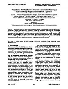
Localization is used in location-aware applications such as navigation, autonomous robotic movement, and asset tracking [1, 2] to position a moving object on a coordinate system. Given three distances from know points, analytical localization methods such as triangulation and trilateration can be used when exact distance measurements can be obtained. In the event that distance measurements are noisy and fluctuate, the task of localizing becomes difficult. This can be seen in Figure 1. With fluctuating distances, regions within the circles become possible locations for the tracked object. As a result, rather than the object being located at a single point, the object can be located anywhere in the dark shaded region in Figure 1. This uncertainty due to the measurement noise renders analytical methods almost useless. Localization methods capable of accounting for and filtering out the measurement noises are desired. Which is why neural networks are very
Permission to make digital or hard copies of all or part of this work for personal or classroom use is granted without fee provided that copies are not made or distributed for profit or commercial advantage and that copies bear this notice and the full citation on the first page. To copy otherwise, to republish, to post on servers or to redistribute to lists, requires prior specific permission and/or a fee. Mobilware’08, February 12-15, 2008, Innsbruck, Austria. c 2008 ACM 978-1-59593-984-5/08/02 ...$5.00. Copyright �
Figure 1: Trilateration with Noise
promising in this area. The method by which the distance measurements are carried out determines the sources of noise in these measurements. Typically devices known as “beacons” are placed at known locations and emit either radio or acoustic signals or both. “Mobile nodes” can determine the distance to a beacon by using the signal strength of the RF signal, Received Signal Strength (RSS) [3]. Other systems utilize both RF and acoustic signals by emitting both at the same time and computing the time difference between their arrival at the mobile node [4, 5, 2, 6]. The Cricket system computes the distance by using the time it takes for the first instance of the acoustic pulse to reach the sensor after the RF signal and the speed at which the acoustic wave typically travels [2, 6]. However, wave reflection is common to both RF and acoustic signals and it is possible that the mobile node erroneously identifies a pulse due to the reflected wave of the original pulse as a new pulse resulting in skewed distance measurements [4]. As a result, the complexity of the methods that can factor these effects increases. However, it must be borne in mind that these methods will be implemented on embedded systems with limited computation and memory resources. Different methods with different levels of accuracy require varying amounts of resources. A trade-off must be made that balances the timely computation of the position and the desired accuracy necessary for the application. With this trade-off in mind, we compare the accuracy, robustness, computational, and memory usage of localization utilizing neural networks with the Position-Velocity (PV) and Position-Velocity-Acceleration models of the Kalman fil-
ters [7]. We will introduce the use of a Radial Basis Function (RBF) neural network for localization, which to our knowledge has not been done before. The rest of the paper is organized as follows. Section 2 describes relevant localization methods. Section 3 introduces principals of neural networks. The experiments by which these methods will be compared are given in Section 4. The results will be discussed in Section 5, and concluding comments will be made in Section 6.
2.
RELATED WORK
The Active Badge Location System [8] is often credited as one of the earliest implementations of an indoor sensor network used to localize a mobile node [2]. Although this system, utilizing infrared, was only capable of localizing the room that the mobile node was located in, many other systems based on this concept have been proposed. The Bat system [4][5], much like the Active-Badge System, also utilizes a network of sensors. This system features a central controller that emits an RF query which the mobile node responds to with an ultrasonic pulse. This pulse is picked up by a network of receivers at varying times due to their locations. These times can be used to compute the distances and hence the location of the mobile node. Researchers at MIT have utilized similar concepts from the Bat System in their Cricket sensors, albeit using a more decentralized structure. This system requires less of a support infrastructure than the Bat system. The Cricket Location System [6] uses a hybrid approach consisting of an Extended Kalman filter, Least Square Minimization to reset the Kalman filter, and Outlier Rejection to eliminate bad distance readings. Other researchers at MIT have proposed localization by exploiting properties of robust quadrilaterals to localize an ad-hoc collection of sensors without the use of beacons [9]. It is also possible to localize optically as shown in the HiBall head tracking system [10]. Arrays of LEDs flash synchronously, and cameras capture the position of these LEDs. The system utilizes information about the geometry of the system and computes the position. Localization using signal strength of RF signals has been studied extensively, [11, 12, 13, 14] are all examples of methods that were devised using this approach. As popular as the Kalman Filter and method involving electromagnetic signals are for localization, neural networks have not been used extensively in this area. There has been some research conducted by Chenna et al in [15]. However, Chenna et al, restricted themselves to comparing Recurrent Neural Networks (RNN) to the Kalman Filter. In [16], we showed that an MLP neural network can be used for localization, and that it’s performance exceeds that of the PV and PVA variants of the Kalman Filter.
3.
INTRODUCTION
In [16], we provide extensive details on the use of Kalman filter for localization. Neural networks are modeled after biological nervous systems and are represented as a network of interconnections between nodes called “neurons” with activation functions. Different classes of neural networks can be obtained by varying the activation functions of the neurons and the structure of the weighted interconnections between them. Examples
of these classes of neural networks are the Multi-Layer Perceptrons (MLP), Radial Basis Function (RBF), and the Recurrent Neural Networks (RNN). The MLP network is “trained” to approximate a function by repeatedly passing the input through the network. The weights of the interconnections are modified based on the difference between the desired output and the output of the neural network. The final weights of the MLP network are entirely dependent upon the initial weights. Finding the set of weights that result in the best performance is a challenge and ultimately becomes a guess and check exercise. The weights of the RBF network are obtained by solving them through the application of Green’s functions [17]. Generally, variations of the Gaussian function are used as activation functions for the nodes. Unlike the MLP network, the weights of the RBF network can be solved for. A major draw back of the RBF neural networks is that it spans the input/output data space of the application, and possibly requires many nodes. Memory and computational requirements of this network can be staggering. However, it is possible to use fewer nodes at key locations to approximate the performance of the much larger network, and thereby significantly reducing memory and computational requirements. These networks are referred to as Reduced RBF (RRBF) networks. RNN networks are very similar to the MLP network structure except in one respect. MLP interconnections only flow from the inputs to the outputs in one direction. There are no connections between the output layers and the previous layers. RNN networks, on the other hand, can posses such a feedback structure. The outputs of a node can be fed back as inputs to previous layers. This unique trait may lend itself well when localization using noisy measurements as will be discussed later. A major benefit of a neural network is that prior knowledge of the noise distribution is not required. Noisy distance measurements can be used directly to train the network with the actual coordinate locations. The neural network is capable of characterizing the noise and compensating for it to obtain the accurate position. Unlike the Kalman filter, which depends upon the knowledge of noise distribution to localize [7]. In any case, the power of neural networks lies in the fact that they can be used to model very complicated relationships easily. Detailed description can be found in [17].
4. EXPERIMENT DESIGN We will explore the performance of the three neural networks described above using MIT Cricket sensors [18]. The distance measurements returned by the sensors are rarely constant and fluctuate often. During our experiment, the measured distances varied by as much as 32.5 cm. The distances from each of the beacons to the mobile node will be used as inputs and the neural networks will output positions that correspond to the location of the mobile node. We will simulate the two dimensional motion of an object by collecting distance measurements of a mobile node while moving it in a network of Cricket sensors. Training data was collected to train the neural networks by utilizing the regular grid of a tile floor where the sensors can be accurately located as shown in Figure 2. Each square tile measures 30 cm wide and lends itself well to the Cricket sensors which can be programmed to measure distance in
centimeters. Using a grid of 300 cm × 300 cm, beacons were placed at positions (0, 300), (300, 300), and (300, 0) of the grid. A representation of this grid can be seen if Figure 3. The training data was collected by placing the mobile node at each intersection of the tiles and collecting distance measurements to each of the three beacons S1 , S2 , and S3 . The distance measurements to the beacons fluctuated constantly, and by collecting more than one set of distances to each of the beacons, we were able to capture the noise in the system. By training the neural networks with these multiple sets of fluctuating distances to beacons for each position, the accuracy of the neural networks improved as it became capable of “filtering” out the noise in the distance measurements. The positions with known locations for which distance measurements were collected are marked using ’+’ signs in Figure 3. For each of the 121 position marked with a “+” sign, several sets of distances measurement were collected resulting in a total of 1521 sets of distance measurements for training the networks.
a linear activation function. This network was trained in MATLAB for 200 epochs with a training goal of 0.001 error. The RNN neural network that will be used is almost the same as the MLP network except that the outputs of the first layer will also be fed back to each of the nodes in the first layer as inputs. Two forms of the RBF network will also be presented: the exact RBF and RRBF. The first layer of the exact RBF network contains 1521 nodes. Each training point has a node associated with it. The RBF network was trained in MATLAB using a variance of 473 until the difference in error between training iterations stabilized. The RRBF network, on the other hand, only has 121 nodes corresponding to the positions where data was collected. All 1521 sets of distances will be used to train the network with a variance of 33. Note that these variances were selected by plotting the localization error of the networks for a variety of different variances and selecting the one that results in the least error.
5. RESULTS AND DISCUSSIONS 5.1 Performance Comparison Figures 4, 5, 6, 10, 11, and 12 show the localization accuracy of the RBF, MLP, RNN, PV, PVA, and RRBF methods respectively. Method RBF MLP RNN PV PVA RRBF
Figure 2: Experiment Test Bed
Locations of Training and Testing Points
Distance Error per Estimate 5.049 5.726 5.738 8.771 9.613 9.998
RMSE (X, Y ) (5.651, 4.582) (5.905, 4.693) (5.936, 4.710) (7.276, 7.537) (8.159, 7.937) (8.177, 11.335)
Net RMSE 7.275 7.543 7.576 10.476 11.382 13.977
300
Table 1: Comparison of Localization Errors (cm) 250
200
150
100
50
0 0
50
100
150
Training Points 200 Testing Points 250
300
Figure 3: Locations of Training and Testing Data Collected Once the training data was collected, the testing data was collected by moving the mobile node through the sensor network following a winding path. Again the distances, for each known positions were collected. This is indicated using the “∗” sign in Figure 3. The distances will be input to the network and they will output estimates of the X and Y coordinates location for those distances. The MLP neural network is a two-layer network composed of nine nodes in the first layer and two nodes in the output layer. The nodes in the first layer use the hyperbolic tangent sigmoid activation function, and the second layer uses
The RBF neural network has the best localization performance according to the average distance error per estimate as given under Distance Error per Estimate in Table 1. This is followed by the MLP, RNN, the PV and PVA model of the Kalman Filter, and then the RRBF neural network. However, a better metric to use is the Root Mean Square Error (RMSE) of the X and Y components of the estimates which reveals the difference, if any, between the X and Y localizations [16]. Our results reveal that the neural networks with the exception of RRBF have a higher percentage of errors of less than 10 cm. Whereas, the Extended Kalman filters have a lower percentage of errors, but most of these errors are greater than 10. Comparing the RBF with the MLP neural network, the MLP network has a lower percentage of errors, but errors of greater magnitude. The RRBF network is also the only method that has error greater than 40 cm, with a spike of about 90 cm. We can also see from Figure 15 this peculiar instance of an extremely large error in the RRBF’s localization at about (267, 260) that significantly affected its RMSE. With significantly fewer nodes spanning the data space, certain locations are not properly accounted for resulting in this singularity.
Testing Points v.s. Localization by RBF NN
Testing Points v.s. Localization by RNN NN
Testing Points v.s. Localization by MLP NN
300
300
300
250
250
250
200
200
200
150
150
150
100
100
100
50
50
50
0
0
0
0
50
100
150
200
Training Points 250 Testing Points RBF NN
300
0
50
100
150
Training Points
200
250
0
300
Testing Points
50
100
150
200
MLP NN
Figure 4: Tracking trajectory of RBF Location of Errors (cm) for RBF Network
Training 250 Points Testing Points RNN NN
300
Figure 5: Tracking trajectory of MLP
Figure 6: Tracking trajectory of RNN
Location of Errors (cm) for MLP Network
Location of Errors (cm) for RNN Network
35
35
40
30
30 30
25
25
20
20
15
10
20 15 10
10
0 300
5
5 250 300
200
0
300
300
250
250
150
250
200 100
200
200
150
150
100
150 100
100
50
50
0
0
Figure 8: Localization errors of MLP
Testing Points v.s. Localization by PV Model Kalman Filter
150
50
0
0
Figure 7: Localization errors of RBF
250 200
200
100
50
100
300 250
150
50
50
0 300
0
Figure 9: Localization errors of RNN Testing Points v.s. Localization by Reduced RBF NN
Testing Points v.s. Localization by PVA Model Kalman Filter
300 300
300
250
250
200
200
150
150
100
100
50
50
250
200
150
0
100
50
0
0 0
50
100
Training Points 250 200
150
300
Testing Points PV Model Kalman Filter
0
50
100
150
Training 200 Points 250 Testing Points PVA Model Kalman Filter
0
300
50
100
150
200
Training Points 250
300
Testing Points RRBF NN
Figure 10: Tracking trajectory of PV
Figure 11: Tracking trajectory of PVA
Locations of Errors (cm) for PV Model Kalman Filter
Locations of Errors (cm) for PVA Kalman Filter
Figure 12: Tracking trajectory of RRBF Location of Errors (cm) for RRBF Network
100 90
35
35
30
80
30
25
70
25
20
60
20
15
15
10
10
5
5
0 300
0 300 250
50 40 30 20 10 250
200
0 300
200 300
150
250 200
100
150
50
100 0
50 0
Figure 13: Localization errors of PV
300 150
250 200
100
150 100
50 0
50 0
Figure 14: Localization errors of PVA
250 200 150 100 50 0
0
50
100
150
200
250
300
Figure 15: Localization errors of RRBF
The RRBF network attempts to approximate the RBF network with fewer nodes, and it comes as no surprise that it’s performance is lower than the RBF’s. A reason why the Kalman filter makes fewer mistakes but larger in magnitude may be due to the process noise of the simulated motion of the object not adhering to the assumptions of Gaussian characteristics [19]. Figures 7, 8, 9, 13, 14, and 15 reveal the location and magnitude of errors in the testing area as shown in Figure 3. It is also interesting to note that the Kalman filters display relatively large errors than the neural networks at the edges of the other boundaries as well. This may be due to the fact that the Kalman filters iteratively close in on the localized position. At the boundaries, where the object’s motion takes a sudden turn, the Kalman filter’s estimates requires several iterations before it can “catch up” with the object, resulting in larger errors. It is also interesting to see that the performance of the MLP and RNN networks is so closely related. The feedback interconnections in this instance does not seem to provide an advantage for the RNN network. However, just like the MLP, the weights associated with the RNN are randomly initialized and trained thereafter, and it is quite possible that for some set of weights, the RNN may indeed function better than the MLP network.
140
120
100
80
60 Actual Kalman PV Kalman PVA MLP RBF RRBF RNN
40
20
0 −50
Figure 17: Equations Method
RBF MLP RNN PV PVA RRBF
0
50
100
150
200
250
Simulated Motion Using Kinematics
Dist Error Per Estimate 16.494 16.568 16.574 23.586 24.845 22.258
RMSE
(13.152, (13.910, (13.900, (16.893, (17.774, (20.225,
10.830) 11.594) 11.622) 17.136) 18.010) 14.330)
Net RMSE 17.037 18.108 18.118 24.063 25.303 24.787
Table 2: RMSE and Sum of Distance Error for Simulated Path Figure 16: Overlapping Error Ranges Associated with Localization Estimates The intuition in using RNN for localization with noisy measurements is that there is an error range associated with each estimate due to the noise. However, it may be possible to reduce this error range by utilizing the past estimate. In Figure 16, the error ranges for estimates P1 and P2 can be seen. However, by utilizing the estimate P1 and its associate error range, the error range for P2 can be narrowed to the intersection of the error range of P1 and P2. The RNN’s feedback mechanisms allow for this behavior. However, in order for this feature to be exploited, the “step size” of the moving object must be small enough that the error ranges overlap. If the step size is too large, as seems to be the case here, the RNN reduces to the MLP network. The “step size” of the moving object here is approximately 30 cm. However, due to the variance of the distance measurements of 32.5 cm, this results in an error range with about radius 16 cm. The step size of this experiment just barely exceeds the error range of each estimate for the features of the RNN network to be useful. In addition to the above analysis, the path of a moving object based on kinematics was simulated. Distances between beacons located at (300, 0), (300, 300), and (0, 300) and a “moving” mobile node were computed. These distances were fed to each of the different localization methods and their performance was analyzed. Figure 17 depicts the estimated path of each of these localization methods. Table 2 reveals that the RBF has the best performance, followed closely by MLP and RNN. There is an interesting paradox in the performance of the RRBF. If the Distance Error Per Estimate
is to be used as a metric, then RRBF performs better than PV. However, if the Net RMSE is to be used as a metric, then RRBF would fall between PV and PVA. Examining the individual X and Y RMSE values, RRBF posses both the worst X localization while possessing the best Y localization among PV, PVA, and RRBF. One of the characteristics of the RMSE is that it is biased towards large errors since large errors squared result in larger values resulting in a greater contribution of error. Due to the unpredictable nature of the RRBF, especially as seen in Figure 15 with the spike in error of about 90 cm, it is best to rank it below the PVA method.
5.2 Computation Comparison Thus far, only the accuracy of the localization methods has been examined without any discussion of the computation requirements associated with them. As mentioned before, these localization methods will be implemented on an embedded system with limited capabilities. Based on the application, an appropriate localization method must be used that balances accuracy with the capabilities of the system. The following analysis utilizes the number of floating point operations as a metric to compare the different methods. For simplicity of presentation, this analysis assumes that the embedded system can perform floating point operations. Further, this analysis only accounts for steady-state computation, meaning the initialization and setup computations are not considered. It is assumed that the neural networks are trained before-hand and the appropriate weights and biases
are available. Method RBF MLP RNN PV PVA RRBF
Number of Floating Point Operations 25857 153 315 884 2220 2057
Table 3: Comparison of Floating Point Operations of Localization Methods Per Estimate As Table 3 reveals, the MLP is the least computationally intensive. It is followed by the RNN, the PV, the RRBF, the PVA, and then finally the RBF. The RBF requires a very large number of floating point operations because of the large number of nodes. These results as described in Table 3 provide an insight into the workings of these localization methods, however, it is very difficult to generalize these results because the size of the neural network may change with different application. The computation of the PV and PVA models of the Kalman filter equations, on the other hand, remains consistent [7]. A two layer MLP, RBF, and RRBF can be implemented using two sets of nested loops. The MLP has complexity O(m2 ) where m is the greatest number of nodes in the two layers. The RNN can also be implemented using two sets of nested loops, however, the complexity changes depending upon the number of nodes in the output layer. The computation at the first layer due to the n2 feedback connections can become the bottle neck for the RNN.
filters with the neural networks. This is because there are no features that are shared between these two families of localizing methods. The neural networks are a more amorphous method of modeling where, in the end, the arrival of the best network for the application is obtained through trial and error. Another reason why it is difficult to arrive at a generalized statement comparing the Kalman filters and the neural networks is because, the scalability of the neural networks is not known. If the area of localization increased from the 300 × 300 cm grid as described above to a 400 × 400 cm grid, the noise characteristics of the distance measurements will also change. The ultrasound signals which are used to measure distances will attenuate differently over this larger distance. The noise characteristic of data for this new area of localization will be different and may require a much larger MLP than the one used above. The Kalman filter does not suffer from the same problem as the neural networks. If the size of the localization area changed, the computation complexity of the Kalman filter will not change.
5.3 Memory Requirement Comparison Comparison of the memory requirements of these localization methods is as problematic as attempting to compare computational complexity. It is not clear at this time how the neural networks will scale compared to the Kalman filter for different applications. In the specific experiment carried out for this paper, the memory usage of the neural networks as compared to the Kalman filters is described in Table 5. It should be noted that the memory usage described here is the steady state memory required. It is also assumed that floats are four bytes long. Method
Method RBF
Order of Magnitude O(m2 )
MLP
O(m2 )
RNN
If (p2 > mn + n2 ), O(p2 ) else, O(mn + n2 )
PV
O(k3 )
PVA
O(k3 )
RRBF
O(m2 )
Comment m is the greater number of nodes in the two layers. m is the greater number of nodes in the two layers. p Output Nodes n Hidden Nodes. m inputs. k is the number of elements in the state variable. k is the number of elements in the state variable. m is the greater number of nodes in the two layers.
Table 4: Comparison of computational complexity between localization methods It is difficult to arrive at a generalized statement comparing the computational complexity of these methods. It is possible to compare the PV and PVA models, and it is possible to compare the MLP, RNN, RBF and RRBF networks. However, there are difficulties in trying to compare Kalman
RBF MLP RNN PV PVA RRBF
Total Memory Usage nm + np + 2n + 2p + m nm + np + 2n + 2p + m n2 + nm + np + 2n + 2p + m 6k2 + 4k + 4km + 5m + m2 6k2 + 4k + 4km + 5m + m2 nm + np + 2n + 2p + m
Number of Bytes 42616 280 604 736 1344 3416
Table 5: Comparison of memory requirements between Localization Methods In the expressions for the two-layer neural networks, n is the number of nodes in the first layer, p is the number of nodes in the output layer, and m is the number of distance readings or the number of inputs. In the expressions for the two Kalman filters, k is the number of elements in the state variable and m is the number of distance readings. The expressions for the memory requirements of the Kalman filters include an additional k2 + 2km + m2 + k + m bytes of memory for temporary variables. Clearly MLP has the least memory usage requirements. It is interesting to note that the underlying memory characteristics for the MLP, RBF, and RRBF are equivalent. This is also true for the Kalman filters. The memory required by the MLP network is less than half of that required by the PV Kalman filter. The large number of nodes spanning the data set results in the increased memory usage for the RBF. The RNN network also suffers due to the n2 feedback
interconnections.
6.
CONCLUSION
The experimental results indicate that among the six localization algorithms, the RBF neural network has the best performance in terms of accuracy. As was mentioned in Section 3, the weights that determine the MLP and RNN neural networks are found by trial and error unlike the weights for the RBF network. The MLP and RNN networks given in this paper were obtained after an extended search. However, it is possible that there may be weights for the MLP and RNN networks that will result in better performance that exceeds the RBF’s. However, as far as the computational and memory requirements are concerned, the MLP is the best. In fact, the MLP’s accuracy is only marginally lower than RBF’s. The MLP neural network offers the best trade-off between accuracy and resource requirements. The RNN neural network also has the potential of exceeding the MLP’s performance if the ”step size” between localization requests are small. It is also apparent that neural networks have a weaker self-adaptivity than the Kalman filters for the following reasons. First, neural networks perform well only for the area in which they have been trained. If the tracked object passes beyond the boundaries of the area where the neural network has been trained, the neural network will not be able to localize. Second, when the beacons from which the distance measurements have been used to train the network are moved, the neural network needs to be re-trained and there is a possibility that the architecture of the neural network may need to change. On the other hand, the Kalman filters do not suffer from this problem and they can be used freely over any area once the appropriate noise parameters have been measured. Compared with Kalman filter methods, the neural networks do have some advantages. The Kalman filters iteratively localize, correcting their estimates over time based on the noise parameters which must be follow a Gaussian distribution. The neural networks on the other hand localize in a single pass of the network. The Kalman filter uses the laws of kinematics to predict the location of the tracked object. If the tracked object’s motion is random and spontaneous the neural network’s ability to localize in a single pass results in more accurate estimates every time. The Kalman filter, however, requires several iterations before it begins to reach the accuracy of the MLP. In conclusion, where noise parameters are not expected to change, the localization method using MLP may be the best option. The high accuracy, minimal computational and memory requirements are highly desirable in embedded systems. If a flexible and easily modifiable method is required, then the Kalman filters may be a better option. However, the decision between the PV and the PVA model of the Kalman filter would depend on the application and the characteristics of the motion of the object.
7.
ACKNOWLEDGMENTS
This work was supported in part by NSF Grants (GK12 #0538457, CCF #0621493, CNS #0723093, and DRL #0737583).
8. REFERENCES [1] Nicholas Roy and Sebastian Thrun. Coastal navigation with mobile robots. In Advances in Neural Processing Systems 12, volume 12, pages 1043–1049, 1999. [2] N. Priyantha. Providing precise indoor location information to mobile devices, 2001. Master’s thesis, Massachusetts Institute of Technology, January 2001. [3] N. Patwari. Location Estimation in Sensor Networks. Ph.d. dissertation, Electrical Engineering, University of Michigan, 2005. [4] A. Ward, A. Jones, and A. Hopper. A new location technique for the active office. In IEEE Personnel Communications, number 5, pages 42–47, October 1997. [5] A. Harter, A. Hopper, P. Steggles, A. Ward, , and P. Webster. The anatomy of a context-aware application. In Proceedings of the 5th Annual ACM/IEEE International Conference on Mobile Computing and Networking (Mobicom ’99), pages 59–68, 1999. [6] A. Smith, H. Balakrishnan, M. Goraczko, and N. Priyantha. Tracking moving devices with the cricket location system. In MobiSys ’04: Proceedings of the 2nd international conference on Mobile systems, applications, and services, pages 190–202, New York, NY, USA, 2004. ACM Press. [7] Yifeng Zhu and Ali Shareef. Comparisons of three Kalman filter tracking models in wireless sensor network. In Proceedings of IEEE International Workshop on Networking, Architecture, and Storages, 2006. NAS ’06., 2006. [8] R. Want, A. Hopper, V. Falc˜ ao, and J. Gibbons. The active badge location system. Technical Report 92.1, Olivetti Research Ltd. (ORL), 24a Trumpington Street, Cambridge CB2 1QA, 1992. [9] D. Moore, J. Leonard, D. Rus, and S. Teller. Robust distributed network localization with noisy range measurements. In SenSys ’04: Proceedings of the 2nd international conference on Embedded networked sensor systems, pages 50–61, New York, NY, USA, 2004. ACM Press. [10] Greg Welch, Gary Bishop, Leandra Vicci, Stephen Brumback, Kurtis Keller, and D’nardo Colucci. High-performance wide-area optical tracking: The HiBall tracking system. Presence: Teleoper. Virtual Environ., 10(1):1–21, 2001. [11] C. Alippi, A. Mottarella, and G. Vanini. A RF map-based localization algorithm for indoor environments. In IEEE International Symposium on Circuits and Systems, 2005. ISCAS 2005., pages 652–655. IEEE CNF, 2005. [12] J. Hightower, G. Borriello, , and R. Want. SpotON: An indoor 3D location sensing technology based on RF signal strength. Technical Report CSE Technical Report NUM 2000-02-02, University of Washington, February 18 2000. [13] K. Lorincz and M. Welsh. A robust decentralized approach to RF-based location tracking. Technical Report TR-04-04, Harvard University, 2004. [14] L. M. Ni, Y. Liu, Y. C. Lau, and A. P. Patil. Landmarc: Indoor location sensing using active RFID. In Proceedings of the First IEEE International Conference on Pervasive Computing and Communications, 2003. (PerCom 2003)., pages 407–415. IEEE CNF, 2003. [15] S. K. Chenna, Y. Kr. Jain, H. Kapoor, R. S. Bapi, N. Yadaiah, A. Negi, V. Seshagiri Rao, and B. L. Deekshatulu. State estimation and tracking problems: A comparison between Kalman filter and recurrent neural networks. In International Conference on Neural Information Processing, pages 275–281, 2004. [16] A. Shareef, Yifeng Zhu, Mohamad Musavi, and Bingxin Shen. Comparison of MLP neural network and kalman filter for localization in wireless sensor networks. In Proceedings of the 19th IASTED International Conference on Parallel and Distributed Computing and Systems, pages 323–330. ACTA Press, 2007. [17] S. Haykin. Neural Networks. Prentice Hall, 1998. [18] Nissanka B. Priyantha, Anit Chakraborty, and Hari Balakrishnan. The cricket location-support system. In MobiCom ’00: Proceedings of the 6th annual international conference on Mobile computing and networking, pages 32–43, New York, NY, USA, 2000. ACM Press. [19] G. Welch and G. Bishop. An introduction to the Kalman filter. Technical Report TR 95-041, University of North Carolina at Chapel Hill, Department of Computer Science, Chapel Hill, NC 27599-3175, 2006.