THE JOURNAL OF CHEMICAL PHYSICS 124, 044911 共2006兲
Brownian dynamics simulations with stiff finitely extensible nonlinear elastic-Fraenkel springs as approximations to rods in bead-rod models Chih-Chen Hsieh,a兲 Semant Jain, and Ronald G. Larson Department of Chemical Engineering, University of Michigan, Ann Arbor, Michigan 48109
共Received 4 October 2005; accepted 28 November 2005; published online 30 January 2006; publisher error corrected 2 February 2006兲 A very stiff finitely extensible nonlinear elastic 共FENE兲-Fraenkel spring is proposed to replace the rigid rod in the bead-rod model. This allows the adoption of a fast predictor-corrector method so that large time steps can be taken in Brownian dynamics 共BD兲 simulations without over- or understretching the stiff springs. In contrast to the simple bead-rod model, BD simulations with beads and FENE-Fraenkel 共FF兲 springs yield a random-walk configuration at equilibrium. We compare the simulation results of the free-draining bead-FF-spring model with those for the bead-rod model in relaxation, start-up of uniaxial extensional, and simple shear flows, and find that both methods generate nearly identical results. The computational cost per time step for a free-draining BD simulation with the proposed bead-FF-spring model is about twice as high as the traditional bead-rod model with the midpoint algorithm of Liu 关J. Chem. Phys. 90, 5826 共1989兲兴. Nevertheless, computations with the bead-FF-spring model are as efficient as those with the bead-rod model in extensional flow because the former allows larger time steps. Moreover, the Brownian contribution to the stress for the bead-FF-spring model is isotropic and therefore simplifies the calculation of the polymer stresses. In addition, hydrodynamic interaction can more easily be incorporated into the bead-FF-spring model than into the bead-rod model since the metric force arising from the non-Cartesian coordinates used in bead-rod simulations is absent from bead-spring simulations. Finally, with our newly developed bead-FF-spring model, existing computer codes for the bead-spring models can trivially be converted to ones for effective bead-rod simulations merely by replacing the usual FENE or Cohen spring law with a FENE-Fraenkel law, and this convertibility provides a very convenient way to perform multiscale BD simulations. © 2006 American Institute of Physics. 关DOI: 10.1063/1.2161210兴 I. INTRODUCTION
The response of dilute solutions of long-chain polymers to imposed flows has been of interest for decades, not only because of its fundamental importance in the characterization of the polymer, but also because of applications such as DNA electrophoresis, DNA microarray analyses, and turbulent drag reduction. To simulate polymer molecules in dilute solutions, molecular-dynamics simulations could be used and quantitative predictions may be obtained. However, it is still far from affordable to simulate with this method a typical polymer or DNA molecule consisting of tens of thousands atoms with numerous surrounding solvent molecules. Fortunately, since the phenomena happening at very short-time 共femtosecond to picosecond兲 and very small length scales 共艋1 nm兲 are not of primary importance for rheological properties of dilute polymer solutions, Brownian dynamics 共BD兲, which is more coarse grained, can be used. Taking advantage of the fact that the configuration relaxation time of a longchain polymer is much longer than its momentum relaxation time, one can replace effectively the velocity distribution of the polymer with a stochastic process with zero correlation a兲
Electronic mail:
[email protected]
0021-9606/2006/124共4兲/044911/10/$23.00
time and thus avoid resolving the very fast dynamics caused by the extremely frequent bombardment of solvent molecules. With Brownian dynamics, linear polymer molecules in dilute solutions are typically modeled by a chain of beads connected by either freely jointed links 共freely jointed chain model兲 or entropic springs 共bead-spring model兲. In the freely jointed chain 共FJC兲 model, a polymer is assumed to remain locally at equilibrium even it has been disturbed at longer length scales. Although the details of the atomic structure of the polymer are lost in such a coarse-grained model, their collective effect can be attributed to the representative length scale of a Kuhn step, which is chosen to be the length of a link in the FJC model. The freely jointed chain model has been shown to reproduce the statistical properties of real polymers on length scales much larger than that of a Kuhn step.1 To simulate a polymer molecule more efficiently, one can use the more coarse-grained bead-spring model in which each entropic spring represents an ensemble of links in the FJC model. The entropic spring force arises from a reduction of the configuration space available to a chain of freely jointed links which is stretched. Consequently, the spring force can be derived from the FJC model and usually can be expressed by a simple function of the stretch of the spring
124, 044911-1
© 2006 American Institute of Physics
044911-2
J. Chem. Phys. 124, 044911 共2006兲
Hsieh, Jain, and Larson
that depends on the degree of the coarse graining.2 Thus, the bead-spring model and the FJC model can be considered equivalent at long-time and long length scales. Both models have been used to simulate DNA/polymer behavior and have been shown to yield results in quantitative agreement with experimental data. More detailed information can be found in recent reviews of Larson3 and Shaqfeh.4 Lately, there is growing interest in understanding the behavior of DNA/polymer near a solid boundary and in microand nanofluidic devices. However, the traditional spring laws that perform well in simulating polymers in bulk flow are no longer valid for such confined chains due to the loss of the configuration space available to the FJC chain. As a result, one should either develop different spring laws for different degrees of confinements5 or use the FJC model instead of the bead-spring model. While the latter method provides a more general solution for BD simulations in confined geometries, it is computationally more expensive than the former method. Therefore, improving the efficiency of the FJC model, especially when hydrodynamic interaction is present, is a key problem that needs to be solved. The freely jointed chain model is usually implemented as the bead-rod model. In the bead-rod model proposed by Kramers,6 a rod represents a rigid link with a fixed length equal to that of a Kuhn step, and a bead is a frictional center. However, the bead-rod model is not the only way to implement a freely jointed chain, and it has been debated whether a stiff Fraenkel spring or a rigid rod is the better choice for simulating the links in a freely jointed chain.7 A Fraenkel spring generates a force proportional to the deviation between the actual spring length and its natural spring length.8 The Fraenkel spring can be so stiff that its length can be kept nearly constant even in a strong flow. Thus, a bead-spring model with Fraenkel springs can be effectively considered as a freely jointed chain. Using this approach, however, in traditional algorithms very small time steps must be used to resolve stably and accurately the rapid change of spring lengths even though one is only interested in the large-scale long-time behavior of the chains. Hence, the bead-rod model has been overwhelmingly preferred over the bead-spring model with stiff Fraenkel springs because much larger time steps can be used with the former without breaking the constraints on rod lengths. However, there are some subtle differences between the bead-rod and the bead-spring models even in the limit of infinite spring stiffness, and the behavior of the bead-spring model with stiff Fraenkel springs is actually closer to that of a freely jointed chain than is the Kramers bead-rod model. Consider, for example, a trumbbell consisting of three beads and two rods. For the bead-spring trumbbell with elastic springs, the probability distribution for the included angle is given by the random-walk configuration,6,9,10 p共兲 = C1 sin共兲.
共1兲
This probability distribution is valid for any elastic spring even in the limit of infinite stiffness. However, Kramers bead-rod trumbbell yields a different probability distribution for the included angle, namely,
p共兲 = C2 sin
冑
1 1 − cos2 , 4
共2兲
where C1 = 0.5 and C2 = 0.522 678 are normalization constants. To retain the random-walk configuration while preserving the efficiency of the bead-rod model, a modified beadrod model that uses an additional pseudopotential to recover the random-walk configuration at equilibrium has been proposed.11–13 However, most workers have simply accepted the deviation from random-walk behavior as appropriate behavior for the Kramers chain.6,14–18 This “traditional” approach has been carried out both with and without hydrodynamic interaction, while the alternative approach, which restores the random-walk configuration, has only been implemented for the free-draining case. In addition to the above issue, constructing a correct Brownian dynamics simulation procedure for the bead-rod model is not trivial. One must be careful to construct the correct stochastic differential equation 共i.e., using Ito’s or Stratonovich’s interpretation; using generalized coordinates or Cartesian coordinates兲 and to choose an appropriate numerical method 共Lagrange multipliers or projection operators兲. Many studies have been criticized because they ignored some subtle issues associated with these methods. The best known algorithm for simulating the freedraining bead-rod chain is the midpoint algorithm proposed by Ryckaert et al.19 and first implemented by Liu.15 In Liu’s method, Lagrange multipliers determined by an iterative scheme are used to enforce constraints on rod lengths. Although everything is evaluated using information obtained at the beginning of each time step, Liu’s algorithm is equivalent to a midpoint algorithm. The advantage of this method is its efficiency. For each iteration, a system of linear equations for the Lagrange multipliers needs to be solved. Since the coefficient matrix is 共nonsymmetrically兲 tridiagonal and constant at each time step over all iterations, the Lagrange multipliers can very efficiently be obtained using backward substitution. The weakness of Liu’s algorithm is in the calculation of the stresses in transient flows, but Doyle et al.17 developed a variance reduction method for the stresses that makes only moderate sacrifice of efficiency. In addition to Liu’s method, a similar algorithm called SHAKE was introduced by Ryckaert et al.,19 in which the Lagrange multipliers are also used to enforce the constraints, but not as efficiently as in Liu’s algorithm. This algorithm is named “SHAKE” because the fulfillment of each constraint partially destroys all previous constraints. Both the midpoint algorithm and the SHAKE algorithm follow the traditional approach 共the Kramers beadrod model兲 and contain no error in their formulation. Besides using the Lagrange multipliers, the constraints can also be fulfilled by a second method using projection operators.13,20–22 In this method, one projects the unconstrained motion of the chain onto the constrained space and thus rejects the motion along the forbidden directions. The drawback of this method is that the trajectory will slowly move away from the constrained space due to the accumulation of the discretization errors and thus will result in a growing deviation in the rod length from its expected value. This
044911-3
J. Chem. Phys. 124, 044911 共2006兲
Brownian dynamics simulations with stiff springs
subtle effect must be suppressed to obtain the correct simulation results.13,21 However, in doing so, care must be taken to avoid introducing additional errors. The advantage of the projection operator is its speed since there is no need for iterations 共although constructing the projection operators is more complicated than carrying out the matrix operations to determine the Lagrange multipliers兲. Although no direct comparison in speed between Liu’s algorithm and the projection-operator method is available in the literature, the latter method should be at least as efficient as the former one. Grassia and Hinch20 followed the approach that recovers the random-walk equilibrium distribution and performed simulations of polymer chain relaxation with the midstep algorithm proposed by Fixman.11 In the midstep algorithm, a predictor step is first used to evaluate the midpoint, and then the second corrector step is performed using the information obtained at the midpoint. A problem in Grassia and Hinch’s algorithm is the way they suppress the numerical drift from the constrained space that leads to an increase in rod length from its natural value. Grassia and Hinch20 and Montesi et al.13 simply rescaled the rod vectors whenever the rod length deviates to a preset upper bound so rod length can be kept nearly constant. However, this simple correction unintentionally alters the equilibrium configuration distribution of the chain and results in a deviation in, for example, equilibrium end-to-end distance and the distribution of the included angles between rods.13,21 This problem becomes more serious when the time step is larger and the simulation is longer. To simulate non-free-draining bead-rod chains, the most widely used algorithm is “SHAKE-HI” originally proposed by Allison and McCammon14 or a variation of it. This algorithm is a straightforward extension of the SHAKE algorithm to include hydrodynamic interaction 共HI兲 and has been used by Agarwal et al.,23 Agarwal,24 Lyulin et al.,25 and Neelov et al.26 Although the SHAKE-HI algorithm may seem correct, it does not reproduce the corresponding kinetic theory.16 First, a metric force arising from the conversion of generalized coordinates to Cartesian coordinates was missed. Second, the constraint conditions are fulfilled at the end of the time step rather than at midpoint. The midpoint and SHAKE algorithms, on the other hand, are correct because, for the free-draining case with identical beads and isotropic mobility tensors, the metric force is canceled, and fulfilling the constraints at the end of the step is equivalent to fulfilling those at the midpoint.Öttinger16 realized these errors and derived correct stochastic differential equations for bead-rod simulations with HI using Ito’s interpretation. Muthukumar and co-workers27,28 implemented Öttinger’s method to simulate a bead-rod chain with hydrodynamic interaction in both shear and extensional flows. In this study, we revisit the approach of using stiff springs to mimic links with constant lengths. With a newly proposed spring law 关the “finitely extensible nonlinear elastic 共FENE兲-Fraenkel spring”兴 and a stable numerical method, the bead-spring model can be efficiently used to simulate a freely jointed chain. The advantages are threefold. First, using a bead-spring model avoids imposing rigid constraints on the rod length and thus avoids the complexity and ambiguity introduced by these constraints. Second, the absence of the
rigid constraints significantly simplifies the calculation of the polymer stresses. Third, existing computer codes for the bead-spring model with nonlinear springs can be trivially switched to simulate the bead-FENE-Fraenkel-spring model and may simplify the development of a multiscale BD simulation platform. This article is organized as follows. In Sec. II, we propose a FENE-Fraenkel spring to replace the Fraenkel spring as an approximation to a rod in the bead-rod model. A stable predictor-corrector method is then adapted for the newly developed bead-FENE-Fraenkel model. In Sec. III, we compare predictions for the Kramers bead-rod model and for the bead-FENE-Fraenkel spring model in equilibrium, relaxation, start-up of uniaxial extensional flow, and steady shear flow in the free-draining limit and steady shear flow in the non-free-draining limit. In Sec. IV we summarize the results and give the conclusions.
II. MODEL A. FENE-Fraenkel spring law
Due to the Hookean nature of the Fraenkel spring, very small time steps have to be used to resolve the fast fluctuations of the spring and to prevent the spring from being overly stretched or compressed. To develop a more efficient algorithm, we need to invent a new spring law and a corresponding implicit numerical method. More specifically, we intend to construct a spring whose length can only fluctuate within a very small range around the value of the rod length Q0 so that the spring behaves similarly to a rigid link in the freely jointed chain. To construct such a spring, we mimic the formulation of the FENE spring law and the Fraenkel spring law, where the former is finitely extensible and the latter has a nonzero equilibrium length. The FENE and the Fraenkel springs are defined by FENE spring:
Fraenkel spring:
F=
HQ , 1 − Q2
F = H共Q − 1兲
共3兲 Q . Q
共4兲
We thus propose a FENE-Fraenkel 共FF兲 spring force law that is very similar to the FENE spring force law but has a nonzero natural length. F=
H共Q − 1兲 Q for共1 − s兲 ⬍ Q ⬍ 共1 + s兲, 1 − 共1 − Q兲2/s2 Q
共5兲
where Q is the spring vector, Q is the spring length, H is the spring constant, and s is the extensibility parameter that defines the maximum possible deviation between the actual spring length and the natural spring length. All variables used in Eqs. 共3兲, 共4兲, and 共5兲, and the following are nondimensionalized using appropriate length and time scales. We follow the common procedure for the bead-rod model17 and choose Q0, Q20 / kBT, and kBT / Q0 as the length, time, and force scales, respectively. Here is the drag coefficient of a
044911-4
J. Chem. Phys. 124, 044911 共2006兲
Hsieh, Jain, and Larson
model. Otherwise, the relaxation spectrum of a freely jointed chain will be truncated by the relaxation time of a spring. This might not be a serious problem when the imposed flow gradient is weak because only the slowest modes are important. However, the criterion for the spring constant must be met when the flow gradient is strong and the fast modes become important. For the FENE-Fraenkel spring, the effective spring constant changes with the stretch of the spring 关see Eq. 共6兲兴, and thus the effective spring constant increases with flow strength. Apart from the above constraint, the value of the spring constant does not have any physical meaning and can be chosen to optimize the numerical method. FIG. 1. The spring force of a FENE-Fraenkel spring vs the spring length with the extensibility parameter s set to be 0.01. Here and all subsequent figures, all quantities are nondimensionalized as described in the text with Q0, Q20 / kBT, and kBT / Q0 as the length, time, and force scales, respectively.
bead and can be related to the bead radius a and the solvent viscosity s by = 6sa. For the FENE-Fraenkel spring, the spring force diverges when the spring length Q approaches either the lower bound 共1 − s兲 or the upper bound 共1 + s兲 so that the spring length is confined between 共1 − s兲 and 共1 + s兲. We illustrate how the spring force changes with the spring extension for different spring constants with s fixed as 0.01 in Fig. 1. As can be seen, the spring length is always confined within the preset range for any spring constant H. The effect of H can be understood by taking the derivative of the spring force F with respect to the spring length Q. That is, dF H关1 + 共1 − Q兲2/s2兴 = . dQ 关1 − 共1 − Q兲2/s2兴2
冦
冋冉
+
冊 冉 冋冉 冊 3R2ij
I+ 1−
冊 册
2a2 RijRij R2ij R2ij
8 3Rij Rij RijRij I+ − 3 4a 4a R2ij
冉 冊 6 ⌬t
1/2 i
ij · n j , 兺 j=1
共8兲
where = ⵜvT is the transpose of the velocity gradient tensor, N is the number of beads, n j is a random vector uniformly distributed in each of three directions over the interval is the 关−1 , 1兴 , ri is the coordinate vector of bead i and Fsp,b j overall spring force acting on bead j. That is, for interior beads, sp = Fsp Fsp,b j j − F j−1 ,
sp sp sp,b Fsp,b 1 = F1 ,FN = − FN .
共7兲
2a2
N
共9兲
is the force that spring j exerts on bead j. For the where end beads,
For the Fraenkel spring, the spring constant H should be chosen so that the spring equilibrates its length faster than a rod equilibrates its orientation in the freely jointed chain
3a Dij = 4Rij Rij 2a
N
dri = · ri + + 兺 · DTij + 兺 Dij · Fsp,b j dt j=1 r j j=1
Fsp j
dF 共Q = 1兲 = H. dQ
1+
We start from Brownian dynamics simulations with hydrodynamic interaction for which the force balance on the ith bead can be described by29
共6兲
At Q = 1, the spring becomes Hookean with
Dii = I,
B. Brownian dynamics simulation with bead-FENEFraenkel-spring model
册
for Rij 艌 2a for Rij ⬍ 2a
共10兲
The diffusion tensor Dij describes the effect of hydrodynamic interaction on bead i induced by a force acting on bead j. For BD simulations, hydrodynamic interaction is usually described by the Rotne-Prager-Yamakawa tensor,30,31
冧
,
i ⫽ j,
共11兲
where Rij is the vector between beads i and j, and Rij = 兩Rij兩. We notice that the hydrodynamic interaction parameter h* is not used in the above expression because its definition is not applied to the bead-rod model which has no “spring length.” From the fluctuation-dissipation theorem, the weighting factor ij in Eq. 共8兲 must satisfy the condition N
Dij = 兺 il · Tjl .
共12兲
l=1
For a given Dij , ij is not unique. Most studies, including the current one, use the Cholesky decomposition, an O共N3兲 scheme, to calculate it.32 A faster spectral approximation method that evaluates the term of ij · n j rather than ij has been proposed
044911-5
J. Chem. Phys. 124, 044911 共2006兲
Brownian dynamics simulations with stiff springs
by Fixman33 and implemented by Jendrejack et al.34 When beads rarely overlap, this approximation scheme roughly scales as N2.25 and is faster than the Cholesky decomposition. However, when beads overlap very frequently, the Cholesky decomposition may be more efficient. The divergence of the diffusion tensor in Eq. 共8兲 arises due to the use of Ito’s interpretation while it will vanish if the Stratonovich interpretation is used instead. In many papers, this term is dropped because it is zero for the widely used Oseen and Rotne-Prager-Yamakawa tensors. However, when a different diffusion tensor is employed or a wall effect is present, this term cannot be neglected. To prevent overstretching or overcompressing the springs, we employ an implicit predictor-corrector method originally designed for the bead-spring model with finitely extensible springs.32,35,36 The key aspect of the predictorcorrector method used here is that for each spring length Q a cubic equation can be constructed that has only one real root between 共1 − s兲 and 共1 + s兲. The FENE-Fraenkel spring law meets the above criterion so the predictor-corrector method can be applied. Since the predictor-corrector method has been described in detail by Somasi et al.36 for the free-draining case and by Hsieh et al.32 for the non-free-draining case, we only briefly summarize the method here. To apply the predictor-corrector method, Eq. 共8兲 has to be rewritten as a function of the spring vectors Q rather than a function of positions of beads r. The predictor step is an explicit Euler integration scheme which provides an initial guess. In corrector steps, spring lengths Q are treated implicitly so that they never become forbidden values. Thus, one obtains the following equation for Qi
冉
1+
冊
B共1 − Qi兲 Qi = Yi , 关s − 共1 − Qi兲2兴Qi 2
共13兲
where we define B = −2s2H⌬t , Yi is actually Ri in Eq. 共3.15兲 of Hsieh et al.,32 and Qi is the magnitude of Qi. By taking the magnitude of each side of Eq. 共13兲, one can reduce it to a set of third-order scalar polynomial equations Q3i − 共2 + Y i兲Q2i + 共2Y i − B + 共1 − s2兲兲Qi + 共Y i共s2 − 1兲 共14兲
+ B兲 = 0.
This cubic equation can be easily solved and always has a unique real root between 共1 − s兲 and 共1 + s兲. Once Qi is obtained, the spring vector can be calculated from Eq. 共13兲 by Qi = Yi
冒冉
1+
冊
B共1 − Qi兲 . 关s − 共1 − Qi兲2兴Qi 2
共15兲
Although this method developed for the earlier bead-spring model can be applied to our new bead-FENE-Fraenkelspring model, care should be taken because the prefactor of Qi in Eq. 共13兲, in contrast to that for ordinary bead-FENEspring model, is not always positive, and its sign cannot be determined before Qi is solved. To guarantee that the correct root is obtained, one should check if Qi obtained from Eq. 共15兲 is consistent with the value of Qi obtained from Eq. 共14兲. If not, one should re-solve Eq. 共14兲 with Y i replaced by −Y i to obtain the correct value of Qi. 共Although without this
FIG. 2. The root Qi of the cubic equation Eq. 共14兲 as a function of the parameter Y i, which is the magnitude of the right-hand side of Eq. 共13兲.
check obtaining the wrong root is possible, this has never happened in our simulations.兲 The corrector steps should be repeated until the residual of Qi has reached a prespecified tolerance. The residual is calculated as the summation of the squares of the differences between the values of Qi obtained from two consecutive iterations. A typical tolerance used in this study for a tenspring chain is 10−7. Using too large a tolerance, such as 10−5, yields wrong equilibrium configurations. In the above procedure, Eq. 共14兲 is solved several times each time step so that a considerable amount of computer time can be saved if one can accelerate this scheme. Since s and B in Eq. 共14兲 are constants for all the springs, any value of Y i corresponds to a unique root 共Qi兲. Figure 2 shows the root of Eq. 共14兲 as a function of Y i given s = 0.01 and ⌬t = 0.001. Since the curve is very smooth, we can build a “lookup table” of roots of Eq. 共14兲 for different values of Y i and use interpolation to obtain approximate solutions instead of solving the cubic equations each time step.21,36 Figure 2 also shows that the value of Qi = 兩Qi兩 is always bounded between 共1 − s兲 and 共1 + s兲. If hydrodynamic interaction is neglected, the diffusion tensor D becomes isotropic and Eq. 共8兲 can be reduced to
冉 冊
6 dri = · ri + Fsp,b + i dt ⌬t
1/2
ni .
共16兲
One can solve Qi the same way as described above. C. Kramers bead-rod model
We will compare simulation results for our bead-FFspring model with those of a Kramers bead-rod model. For the free-draining case, Liu’s algorithm will be used to generate results of bead-rod model for comparison. We refer the readers to Liu15 and Doyle et al.17 for more details about the algorithm. All simulation results presented here for the freedraining case use ten-spring 共rod兲 chains with a contour length of ten dimensionless units. We note that the definition of the tolerance for the bead-FF-spring model is different from that for the bead-rod model. For the bead-rod model, we use
044911-6
J. Chem. Phys. 124, 044911 共2006兲
Hsieh, Jain, and Larson Ns
= 兺 共Qi − 1兲2 .
共17兲
i=1
For ten-spring 共rod兲 chains, the tolerance is set to 10−7 for both models, if not specified otherwise. Since developing an algorithm for the bead-rod model with hydrodynamic interaction is not trivial and also not the main goal of this study, we choose to compare our results for shear flow with HI to those obtained by Petera and Muthukumar,27 who implemented Öttinger’s algorithm.16 D. Evaluation of stress
For the bead-FENE-Fraenkel spring model, we calculate the polymer stresses from Ns
= 兺 具Fsp i Qi典.
共18兲
i=1
For the bead-rod model, the stress is calculated using the Kramers-Kirkwood expression, N+1
= 兺 具RiFHi 典,
共19兲
i=1
where is the number density of polymer chains and is set to unity in this study, Ri is the position vector of bead i and FH i is the hydrodynamic force acting on bead i which can be calculated as the negative summation of the Brownian and constraint forces. In this study, no variance 共or noise兲 reduction technique is used for either model. However, we point out that the variance reduction techniques developed for the regular bead-spring model, such as the control variate method35,37 can be applied to the bead-FF-spring model without any modification. E. Initial configuration and general setup
As will be shown later, the bead-FF-spring model yields a random-walk configuration at equilibrium, so we can easily generate initial equilibrium configurations. To obtain initial configurations for the bead-rod model, we start from a random-walk configuration and run the simulation under a no-flow condition. We discard the results obtained in the initial period of 200 relaxation times and then record the configuration of the polymer chain once every two relaxation times until enough configurations are obtained. III. RESULTS AND DISCUSSION A. Choosing spring constant H and extensibility parameter s
As mentioned above, the spring constant H does not have a physical meaning and the choice of the value of H can be solely based on minimizing computer time. To demonstrate this, we first test the influence of H on the equilibrium end-to-end distance squared for value of H ranging from 100 to 1 000 000 with s = 0.01 and time step ⌬t = 0.001. The simulated equilibrium end-to-end distance squared is an average over a period of 100 000 relaxation times and deviates
FIG. 3. Comparison of the average value of 11 vs time in start-up of extensional flow for different values of H at Weissenberg number Wi= 10. The inserted plot is a histogram of 11,plateau − 具11,plateau典.
less than 0.3% from its expected value. Thus, H has negligible effect on the equilibrium end-to-end distance squared. We next test the influence of H on the polymer stresses in a start-up uniaxial extensional flow. In Fig. 3, we compare the simulated 11 versus time in transient extensional flow with Weissenberg number Wi= 10 for different values of the spring constant H. The Weissenberg number Wi is defined as the product of the strain rate and the longest relaxation time of the chain. The relaxation time is evaluated using Eq. 共20兲 that will be introduced in a later section. Each curve in Fig. 3 represents an ensemble average of 10 000 independent runs. The time step ⌬t and extensibility parameter s are set to 10−4 and 0.01, respectively. Although different values of H are used, the simulation results are essentially the same. We then analyze the degrees of fluctuation of 11 after it reached the steady state. The results are shown as a histogram of 11,plateau − 具11,plateau典 in the insert of Fig. 3. We find that 11,plateau is much noisier for simulations using H = 106 than for those using H = 102 and H = 104. The latter two have essentially the same magnitude of noise. The computational costs are 6.5, 6.4, and 8.1 iterations per step for H = 102, 104, and 106, respectively. We thus confirm that any reasonable choice of H is safe while there is an optimum range of H that can keep the computational cost low. For the simulations in this study for a ten-spring chain, a rule of the thumb we find is that H = 1000Wi. A more general method for choosing an appropriate value of H is to perform a test run. One can choose any value of H for the test run and compute the approximate average spring force 具F典. H can then be chosen by setting H ⬃ 1.5具Fsp典 / s which implies that the average deviation in the spring length from its natural length 共i.e., the rod length兲 is around 0.5s. The extensibility parameter s determines the maximum and minimum spring lengths. If s is very small, the spring becomes very stiff and a large number of iterations are required to achieve convergence. On the other hand, using a large value of s results in a large deviation in the spring length Q from the natural spring length. We test the influence of the extensibility parameter s using free-draining BD simulation of a chain in a start-up uniaxial extensional flow and
044911-7
J. Chem. Phys. 124, 044911 共2006兲
Brownian dynamics simulations with stiff springs
FIG. 4. Comparison of the average value of 11 vs time in start-up extensional flow with different values of s at Weissenberg number Wi= 10. The inserted plot is magnification of this plot over a small time window in the plateau region.
show the simulated 11 versus time in Fig. 4. Each curve in Fig. 4 represents an ensemble average of 10 000 independent runs. The time step ⌬t and the spring constant H are set to be 10−4 and 104, respectively. The inserted plot is an enlarged view of the stress plateau. As can be seen, when s becomes smaller, the simulation results converge on average although noise increases for smaller s. The average iterations per step are 6.4, 7.6, and 12.0 for s = 0.05, s = 0.01, and s = 0.001, respectively. Although the simulation is fastest for s = 0.05, this value leads to an inaccurate plateau value of 11 due to the large deviation in the spring length from its natural length. We therefore use s = 0.01 for the following simulations because it provides an acceptable result at a reasonable computational cost.
FIG. 5. The probability distribution for the included angle of a trumbbell. Solid lines represent the theoretical predictions and dashed lines the simulations results. The gray lines were obtained using the bead-rod model and black lines using the bead-FF-spring model. The parameters for the beadFF-spring model are s = 0.01, H = 1000, and ⌬t = 0.0001.
1 = 0.0142共Ns + 1兲2 .
共20兲
This will be used to calculate the Weissenberg numbers for both the bead-FF-spring and the bead-rod models in the following. 2. Start-up of uniaxial extensional flow
1. Equilibrium and relaxation
Figure 7 compares predictions of 11 for the bead-rod model with the midpoint algorithm to that of the bead-FFspring model with the predictor-corrector method after start-up of uniaxial extensional flow at Wi= 10. Each curve is an average over 1000 individual runs. Only one time step ⌬t = 0.001 is used for the bead-rod model because it does not converge if a larger time step is employed. Actually, even with ⌬t = 0.001, the bead-rod simulations often become unstable after ten dimensionless time units 共or roughly 60 strain units兲. Therefore, this is the largest time step allowed for bead-rod model simulations with the specified tolerance. On
We first perform simulations at an equilibrium state to verify that the bead-FF-spring model yields a random-walk configuration. Figure 5 compares the simulation results of the bead-rod model and the bead-FF-spring model consisting of three beads and two rods with theoretical predictions for the included angle. The bead-FF-spring model yields a random-walk configuration while bead-rod model does not. Both models yield probability distributions in agreement with the theoretical predictions given by Eqs. 共1兲 and 共2兲. Figure 6 plots the square of the stretch 具x2典 simulated by the bead-rod model and the bead-FF-spring model versus time. We start from a fully stretched configuration and run the simulations under a no-flow condition until the chains are completely relaxed. Each curve is an ensemble average of 500 runs. As can be seen, the two curves almost overlap perfectly with each other. Therefore, we can infer that the two models give very similar relaxation times. For convenience, the longest relaxation time 1 for the bead-rod model in the free-draining limit will be estimated using the formula provided by Doyle et al.,17
FIG. 6. Comparison of relaxation of stretch square for of a ten-rod 共spring兲 chain vs time for the bead-rod model with Liu’s algorithm and the bead-FFspring model with the predictor-corrector method. Each curve represents an ensemble of 500 independent runs. Hydrodynamic interaction is not included.
B. The bead-FENE-Fraenkel-spring model versus the bead-rod model in the free-draining limit
044911-8
J. Chem. Phys. 124, 044911 共2006兲
Hsieh, Jain, and Larson
FIG. 7. Comparison of polymer contribution to 11 vs time in start-up extensional flow with Weissenberg number Wi= 10 for the bead-rod model with Liu’s algorithm and the bead-FF-spring model with the predictorcorrector method. Each curve is an average over an ensemble of 1000 runs. Hydrodynamic interaction is not included. The inserted plot shows an enlarged view of the fluctuation about the plateau value of 11.
the other hand, the bead-FF-spring model is very stable even with ⌬t = 0.005. We therefore present results for both ⌬t = 0.005 and ⌬t = 0.001. It can be observed that both methods predict a very similar value of 11. However, the bead-FFspring model yields an ensemble average value of 11 with smaller fluctuations 共see the inserted plot of Fig. 7兲. Figure 8 shows the histogram of the deviation between the instantaneous value of 11,plateau and its average value 具11,plateau典. We assume that 11 reaches its plateau after t = 3 共17.5 strain units兲 and collect data at every time step between t = 3 to t = 4 in each realization until 2 ⫻ 106 data points are obtained. From Fig. 8, we observe two trends. First, using a larger time step effectively reduces the noise in the prediction of stresses for the bead-FF-spring model. Second, the bead-FF-model yields a narrower distribution of 11,plateau − 具11,plateau典 than does the bead-rod model when the same time step and tolerance are used. The standard errors of the mean of these data are 0.267, 0.160, and 0.091 for the bead-rod model with ⌬t = 0.001, the bead-FF-spring model with ⌬t = 0.001, and the bead-FF-
FIG. 9. Comparison of steady-state shear viscosity scaled with the zeroshear viscosity vs Weissenberg number in shear flow for the bead-rod model with Liu’s algorithm and the bead-FENE-Fraenkel-spring model with the predictor-corrector method. Hydrodynamic interaction is not included.
spring model with ⌬t = 0.005, respectively. The absolute values of the standard errors of the mean are very small because we collect a large set of data. Since the standard error of the mean decreases proportionally to the square root of the number of the samples, we can infer that only about one-third of realizations are needed for the bead-FF-spring model with time step ⌬t = 0.001 to obtain the results with the same accuracy as those of the bead-rod model provided that the time step and the tolerance are the same. Furthermore, because the bead-FF-spring model allows a larger time step, ⌬t = 0.005, it needs about only one-eighth of realizations to obtain results with the same accuracy as those of the bead-rod model with ⌬t = 0.001. 3. Steady shear flow
In Fig. 9, we compare the polymer contribution to the shear viscosity obtained using the bead-FF-spring model with that using the bead-rod model in steady shear flow versus the Weissenberg number Wi averaged over at least 20 000 strain units. The Weissenberg number for shearing flow is defined as the product of the longest relaxation time and the shear rate. The parameters are listed in Table I. We note that the simulation parameters are not optimized, but each result is verified using an additional set of simulations with a smaller tolerance and smaller time step. In shear flow, the bead-FF-spring model does not have the advantage of TABLE I. Simulation parameters for the bead-rod model and the beadFENE-Fraenkel-spring model in shear flows. Bead-rod model Wi
FIG. 8. Histogram of the deviation between the instantaneous value of 11, plateau and its average value 具11, plateau典.
0.1 1 10 100 1 000 10 000 100 000
⌬t −3
10 10−3 10−3 3 ⫻ 10−4 10−4 10−5 10−6
Bead-FENE-Fraenkel-spring model H 3
10 103 104 104 2 ⫻ 104 105 106
s
⌬t
0.01 0.01 0.01 0.01 0.01 0.01 0.01
10−3 10−3 10−3 3 ⫻ 10−4 10−4 10−5 10−6
044911-9
J. Chem. Phys. 124, 044911 共2006兲
Brownian dynamics simulations with stiff springs
FIG. 10. Comparison of steady-state shear viscosity vs Weissenberg number in shear flow for the bead-rod model and the bead-FENE-Fraenkel-spring model. Hydrodynamic interaction is included.
allowing larger time steps. The shear viscosities shown in Fig. 9 are normalized using the zero-shear viscosity given by 共共Ns + 1兲2 − 1兲 / 36.8 As can be seen, the two models once again generate very similar results. We also check the standard errors of the mean M of the shear viscosities generated by both models and find that the ratio of M,bead-FF-spring to M,bead-rod is 0.9. Thus, the bead-FF-spring model predicts slightly less noisy shear stresses than does the bead-rod model. C. The bead-FENE-Fraenkel-spring model versus the bead-rod model with hydrodynamic interaction
Since developing a BD code for the bead-rod model with hydrodynamic interaction is not trivial and also is not the main interest of this study 共in fact, part of our purpose in developing the FF spring is to avoid needing to develop a bead-rod model with HI兲, we choose to compare our simulation results with those of Petera and Muthukumar.27 A 20rod chain was used for their simulations in shear flow. The hydrodynamic radius a is taken from Petera and
Muthukumar27 and is set to be 0.5. Figure 10 compares the predicted shear viscosities from both models. All results represent averages over at least 200 000 dimensionless time units. From Fig. 10, it is a little surprising that there seems to be a discrepancy between the predicted shear viscosities given that two models predict very similar results for the free-draining case. However, we need more data for comparison to determine if this discrepancy is generic or merely caused by inaccurate simulations. Since bead-rod simulations with HI are complicated to formulate and implement while with the FENE-Fraenkel spring, there is no added complication beyond that of a normal bead-spring chain, we believe that if a formulation or coding error is responsible for the difference in Fig. 10, the error is more likely to reside in the code for the bead-rod chain than in that for the bead-FFspring chain. D. Efficiency of the bead-FF-spring model
For the free-draining bead-FF-spring model, the computational cost per time step scales roughly linearly with the number of springs Ns if the time step does not change with Ns. This scaling is the same as that for the bead-rod model with the midpoint algorithm, the SHAKE algorithm, or projection operators. Because of the iterative nature of the predictor-corrector method, the number of iterations differs in each step and also changes with the choice of parameters. Therefore, the scaling provided is only a rough guide, not a precise result. Table II shows the computer times corresponding to Fig. 7 as well as those for simulating the equilibrium state. Each set of data represents the computer time for simulating a ten-spring 共rod兲 chain over an ensemble of 2000 runs with 4000 steps in each run for those with ⌬t = 0.001 and with 800 steps for those with ⌬t = 0.005. The programs were implemented in FORTRAN 90, compiled with PGI FORTRAN compiler 3.2, and run on an Intel Pentium III 1.0 GHz processor. From Table II, we can estimate that the computational cost per time step for a free-draining BD simulation with the proposed bead-FF-spring model is about twice as high as the
TABLE II. Comparison of computational time per time step for the bead-rod model with Liu’s algorithm and the bead-FENE-Fraenkel model with the predictor-corrector method. Start-up of extensional flow 共Wi= 10兲
At equilibrium
CPU time 共s兲 Bead-rod model with Liu’s algorithm, ⌬t = 0.001 Bead-FF-spring with predictorcorrector method ⌬t = 0.001 Bead-FF-spring with predictorcorrector method ⌬t = 0.005
Number of iterations
Average error in rod length
CPU time 共s兲
Number of iterations
Average error in rod length
93
5.32
6.41E − 4
110
6.22
6.84E − 4
187
6.15
2.30E − 3
212
7.00
4.14E − 3
43
7.07
1.29E − 3
53
8.92
4.12E − 3
044911-10
J. Chem. Phys. 124, 044911 共2006兲
Hsieh, Jain, and Larson
traditional bead-rod model with the midpoint algorithm of Liu15 for a given time step and tolerance. However, the beadFF-spring model can be as efficient because it allows use of a larger time step and it yields less noisy results as demonstrated earlier. If the hydrodynamic interaction is included, the computer time is dominated by the decomposition of the diffusion tensor D which scales roughly as 共Ns + 1兲3. Therefore, the bead-FF-spring model should be faster for extensional flow because it allows larger time steps. IV. CONCLUSIONS
We propose to use the bead-spring model with stiff FENE-Fraenkel springs as an alternative to the bead-rod model for simulating freely jointed chains in Brownian dynamics simulations. We developed a FENE-Fraenkel spring that is finitely extensible and has a natural length equal to the rod length in the bead-rod model. A predictor-corrector method originally developed for the bead-spring model was developed and tested. In the free-draining limit, we compared results from BD simulations of the bead-FENEFraenkel-spring model against those for the bead-rod model in relaxation, steady-state shear, and start-up of extensional flow and find that both methods generate very similar results. Both models are also comparably efficient in use of computer time. When hydrodynamic interaction is included, a slight discrepancy is observed between the predicted shear viscosities. However, more data are needed for a more detailed comparison. Summarizing the above findings, we conclude that the bead-FENE-Fraenkel-spring model can be used as an alternative method to simulate a freely jointed chain. With this new model, existing computer codes for bead-spring models can trivially be converted to ones for effective bead-rod simulations merely by replacing the usual FENE or Cohen spring law with a FENE-Fraenkel law. This convertibility provides a very convenient way to perform multiscale BD simulations. ACKNOWLEDGMENTS
This material is based upon work supported in part by the National Science Foundation under Grant No. NSF DMR-0072101. Any opinions, findings and conclusions or recommendations expressed in this material are those of the
authors and do not necessarily reflect the views of the National Science Foundation 共NSF兲. The authors also thank Professor David D. Morse for helpful discussions. P. J. Flory, Statistical Mechanics of Chain Molecules 共Oxford University Press, New York, 1988兲. 2 P. T. Underhill and P. S. Doyle, J. Rheol. 49, 963 共2005兲. 3 R. G. Larson, J. Rheol. 49, 1 共2005兲. 4 E. S. G. Shaqfeh, J. Non-Newtonian Fluid Mech. 130, 1 共2005兲. 5 N. J. Woo, E. S. G. Shaqfeh, and B. Khomami, J. Rheol. 48, 281 共2004兲. 6 H. A. Kramers, J. Chem. Phys. 14, 415 共1946兲. 7 J. M. Rallison, J. Fluid Mech. 93, 251 共1979兲. 8 R. B. Bird, C. F. Curtiss, R. C. Armstrong, and O. Hassager, Dynamics of Polymeric Liquids 共Wiley-Interscience, New York, 1987兲, Vol. 2. 9 O. Hassager, J. Chem. Phys. 60, 2111 共1974兲. 10 M. Gottlieb and R. B. Bird, J. Chem. Phys. 65, 2467 共1976兲. 11 M. Fixman, J. Chem. Phys. 69, 1527 共1978兲. 12 E. J. Hinch, J. Fluid Mech. 271, 219 共1994兲. 13 A. Montesi, D. C. Morse, and M. Pasquali, J. Chem. Phys. 122, 084903 共2005兲. 14 S. A. Allison and J. A. McCammon, Biopolymers 23,167 共1984兲. 15 W. T. Liu, J. Chem. Phys. 90, 5826 共1989兲. 16 H.-C. Öttinger, Phys. Rev. E 50, 2696 共1994兲. 17 P. S. Doyle, E. S. G. Shaqfeh, and A. P. Gast, J. Fluid Mech. 334, 251 共1997兲. 18 J. S. Hur, E. S. G. Shaqfeh, and R. G. Larson, J. Rheol. 44, 713 共2000兲. 19 J. P. Ryckaert, G. Ciccotti, and H. J. Berendsen, J. Comput. Phys. 23, 327 共1977兲. 20 P. S. Grassia and E. J. Hinch, J. Fluid Mech. 282, 373 共1995兲. 21 E. A. J. F. Peters, Ph.D. thesis, Delft University of Technology, 2000. 22 D. C. Morse, Adv. Chem. Phys. 128, 65 共2004兲. 23 U. S. Agarwal, R. Bhargava, and R. A. Mashelkar, J. Chem. Phys. 108, 1610 共1998兲. 24 U. S. Agarwal, J. Chem. Phys. 113, 3397 共2000兲. 25 A. V. Lyulin, D. B. Adolf, and G. R. Davies, J. Chem. Phys. 111, 758 共1999兲. 26 I. M. Neelov, D. B. Adolf, A. V. Lyulin, and G. R. Davies, J. Chem. Phys. 117, 4030 共2002兲. 27 D. Petera and M. Muthukumar, J. Chem. Phys. 111, 7614 共1999兲. 28 S. Liu, B. Ashok, and M. Muthukumar, Polymer 45, 1383 共2004兲. 29 D. L. Ermak and J. A. McCammon, J. Chem. Phys. 69, 1352 共1978兲. 30 J. Rotne and S. Prager, J. Chem. Phys. 50, 4831 共1969兲. 31 H. Yamakawa, J. Chem. Phys. 51, 436 共1970兲. 32 C. -C. Hsieh, L. Li, and R. G. Larson, J. Non-Newtonian Fluid Mech. 113, 141共2003兲. 33 M. Fixman, Macromolecules 19, 1195 共1986兲. 34 R. M. Jendrejack, M. D. Graham, and J. J. de Pablo, J. Chem. Phys. 113, 2894共2000兲. 35 H.-C. Öttinger, Stochastic Processes in Polymeric Fluids 共Springer, Berlin, 1996兲. 36 M. Somasi, B. Khomami, N. J. Woo, J. S. Hur, and E. S. G. Shaqfeh, J. Non-Newtonian Fluid Mech. 108, 2275共2002兲. 37 M. Herrchen and H.-C. Öttinger, J. Non-Newtonian Fluid Mech. 68, 17 共1997兲. 1