Nov 22, 2004 - and Williams-Watt models have been developed to describe ... subject to AIP license or copyright, see http://jcp.aip.org/jcp/copyright.jsp ...
JOURNAL OF CHEMICAL PHYSICS
VOLUME 121, NUMBER 20
22 NOVEMBER 2004
Fractional Brownian dynamics in proteins G. R. Kneller Laboratoire Le´on Brillouin, CNRS, F-91191 Gif-sur-Yvette, France and Centre de Biophysique Mole´culaire, CNRS, Rue Charles Sadron, F-45071 Orle´ans Cedex 2, Francea兲
K. Hinsen Laboratoire Le´on Brillouin, CNRS, F-91191 Gif-sur-Yvette, France
共Received 6 May 2004; accepted 19 August 2004兲 Correlation functions describing relaxation processes in proteins and other complex molecular systems are known to exhibit a nonexponential decay. The simulation study presented here shows that fractional Brownian dynamics is a good model for the internal dynamics of a lysozyme molecule in solution. We show that both the dynamic structure factor and the associated memory function fit well the corresponding analytical functions calculated from the model. The numerical analysis is based on autoregressive modeling of time series. © 2004 American Institute of Physics. 关DOI: 10.1063/1.1806134兴
I. INTRODUCTION
Relaxation processes in complex dynamical systems, ranging from glasses to proteins, have attracted considerable interest for more than 50 years. Complexity manifests itself in the presence of a large quasicontinuous spectrum of relaxation rates of the dynamical variables under consideration. As a result, the corresponding time correlation functions exhibit a strongly nonexponential decay. The Cole-Davidson and Williams-Watt models have been developed to describe this phenomenon in the context of dielectric relaxation measurements.1,2 A comparative study can be found in a later paper by Lindsey and Patterson,3 and Zeidler discusses a unified model from a mathematical point of view.4 Nonexponential behavior of time correlation functions can also be observed in reaction kinetics.5 Some years ago, Glo¨ckle and Nonnenmacher suggested the model of fractional Brownian dynamics 共FBD兲 to describe ligand rebinding in myoglobine upon flash photolysis.6 Essentially, FBD is a model where the stochastic displacement of normal BD, which is described by a Wiener process, is replaced by a convolution of the latter with an algebraic kernel. In this way memory effects are introduced, which are absent in classical Brownian motion. The FBD model has been applied to describe the time evolution of such different systems as water reservoirs and stock markets. For an introduction we refer to an early paper by Mandelbrot and van Ness and references therein.7 Recently Schiessel et al. demonstrated that the FBD model arises naturally in polymer dynamics as a consequence of the viscoelastic properties of polymers and polymer networks.8 The reaction kinetics of ligand 共re兲 binding is effectively a probe for the internal dynamics of proteins which is characterized by a strong coupling between fast vibrational motions of single bonds, less rapid rotational motions of sidechains, and slow motions of the backbone. The strong coupling of these different types of motions leads to a broad a兲
Affiliated with the University of Orle´ans.
0021-9606/2004/121(20)/10278/6/$22.00
spectrum of relaxation rates, ranging from sub-picoseconds to seconds. A model for protein dynamics which is borrowed from reaction kinetics has been proposed by Frauenfelder and co-workers.9,10 Within this model one considers a ‘‘rugged’’ energy landscape with many conformational substates. Transitions between these substates are thermally activated and occur with frequencies which are related to the barrier heights. Using the picture of a fractal protein energy landscape, Carlini et al. have recently examined the nonLorentzian form of the Fourier-transformed time autocorrelation function of the potential energy of the plastocyanine protein. They show that their results are compatible with the FBD model.11 We show in this paper that the FBD model can also be used to describe the collective internal dynamics of a protein in solution, as it is seen through the dynamic structure factor, which can also be measured by quasielastic neutron scattering. Not only the coherent dynamic structure factor is well described by the model, but also the memory function which is associated with the corresponding time correlation function. The fact that the characteristic form of the model memory function can also be extracted from the simulated trajectories yields additional evidence for the validity of the FBD model. The concept of memory functions was introduced by R. Zwanzig in order to derive a systematic equation for the time evolution of time correlation functions.12 It has been extensively used in order to derive analytical models,13 and a method to compute memory functions of time correlation functions from molecular dynamics 共MD兲 simulations has been published recently.14,15 The paper is organized as follows: In the following section we present first the essential properties model of the FDB model. Starting from the Laplace transform of the corresponding time correlation function, we derive its Fourier spectrum and the associated memory function. In the third section we present first briefly the numerical calculation of the latter and show then the results obtained from molecular
10278
© 2004 American Institute of Physics
Downloaded 05 Apr 2007 to 195.221.0.6. Redistribution subject to AIP license or copyright, see http://jcp.aip.org/jcp/copyright.jsp
J. Chem. Phys., Vol. 121, No. 20, 22 November 2004
Fractional Brownian dynamics in proteins
10279
dynamics of a lysozyme molecule in solution. The last section is devoted to the discussion of the results. II. FRACTIONAL BROWNIAN DYNAMICS A. Correlation function
In this section we review briefly the essential properties of the correlation function associated with the FBD model. For more details we refer to the paper by Glo¨ckle and Nonnenmacher6 and the references therein, in particular, the book on higher transcendental functions by Erde´lyi et al.16 and the book by Oldham and Spanier on fractional calculus.17 Within the FBD model the normalized autocorrelation function of a time dependent variable has the form (t ⭓0)
FBD共 t 兲 ⫽E  关 ⫺ 共 t/ 兲  兴 ,
0⬍  ⭐1,
共1兲
where E  (z) is the Mittag-Leffler function,16 ⬁
E 共 z 兲 ⫽
zk . ⌫ 共 1⫹  k 兲
兺
k⫽0
共2兲
As usual, ⌫(z) denotes the Gamma function.18 An important property of FBD(t) is its algebraic decay for long times,
FBD共 t 兲 ⬀
冉冊 t
⫺
,
tⰇ , 0⬍  ⬍1,
共3兲
which follows from the properties of the Mittag-Leffler function.16 The model correlation function is the solution of the fractional differential equation17 t ⫺  ⫺ Dt 共 t 兲⫹ 共 t 兲⫽ , ⌫ 共 1⫺  兲
共4兲
where the initial condition is incorporated.6 D t represents a fractional derivative of order , D t f 共 t 兲 ª
dn dt
D  ⫺n f 共 t 兲 . n t
共5兲
FIG. 1. The solid line shows FBD(t), as defined by Eq. 共2兲, for ⫽1/2. For comparison the exponential function, exp关⫺(t/)兴, and the stretched exponential, exp关⫺(t/)兴 are shown 共long dashes and dot-dashed line, respectively兲. The inset shows the memory function defined by Eqs. 共15兲 and 共21兲, with ⫽1/2, ⫽1, and ⑀⫽0.1. The vertical line indicates the region where (t) has the form 共21兲.
SE共 t 兲 ⫽exp关 ⫺ 共 t/ 兲  兴
for ⫽1/2. It should be noted that SE(t) is obtained from Eq. 共1兲 by replacing the Mittag-Leffler function by a normal exponential function.
B. Fourier spectrum of the correlation function
Since the series 共2兲 converges slowly with increasing 兩 z 兩 , the numerical calculation of FBD(t) is difficult if tⰇ . In contrast to FBD(t) its Laplace transform has a simple analytical form
冕
t
0
d
共 t⫺ 兲 ␣ ⫺1 f 共 兲. ⌫共 ␣ 兲
共6兲
For special values of , the correlation function FBD(t) can be written as a closed expression. For ⫽1 one retrieves the exponential function FBD(t)⫽exp关⫺(t/)兴, and Eq. 共4兲 becomes d共 t 兲 ⫹ ⫺1 共 t 兲 ⫽ ␦ 共 t 兲 . dt
共7兲
The appearence of the right-hand sides in Eqs. 共7兲 and 共4兲 is due to the fact that 共fractional兲 derivatives are to be considered as left-hand derivatives. This point will become clear in the following section. For ⫽1/2 the Mittag-Leffler function can be expressed in closed form,16 and one obtains for the correlation function FBD(t)⫽exp关(t/)兴erfc关(t/)1/2兴 . Figure 1 shows FBD(t) for ⫽1 共exponential function兲 and for ⫽1/2, as well as the ‘‘stretched’’ exponential function,2
冕
ˆ FBD共 s 兲 ⫽
␣ Here ⬎0, n is the nearest integer to  with n⭓  , and D ⫺ t 共␣⭓0兲 denotes a fractional integration of order ␣, ␣ D⫺ t f 共 t 兲⫽
共8兲
⬁
0
dt exp共 ⫺st 兲 FBD共 t 兲 ⫽
0⬍  ⭐1,
1 s 关 1⫹ 共 s 兲 ⫺  兴
兩 s 兩 ⬍1.
, 共9兲
The above expression can be used to derive the Fourier spectrum of FBD(t). Since autocorrelation functions are even in time if the underlying stochastic process is 共wide-sense兲 stationary, it follows that S FBD( )⫽lim⑀ →0⫹ 2Rˆ FBD( ⑀ ⫹i ). Stationarity can be assumed for any time correlation describing a system in thermal equilibrium. Using expression 共9兲 one obtains thus S FBD共 兲 ⫽
2 sin共  /2兲 
兩 兩 共 兩 兩 ⫹2 cos共  /2兲 ⫹ 兩 兩 ⫺  兲
0⬍  ⭐1.
, 共10兲
For ⫽1 one retrieves a Lorentzian S共 兲⫽
2 1⫹ 共 兲 2
.
共11兲
Downloaded 05 Apr 2007 to 195.221.0.6. Redistribution subject to AIP license or copyright, see http://jcp.aip.org/jcp/copyright.jsp
10280
J. Chem. Phys., Vol. 121, No. 20, 22 November 2004
G. R. Kneller and K. Hinsen
sponds to the correlation function given by Eq. 共2兲. For this purpose we compare expression 共9兲 to the Laplace transform of the memory function equation 共14兲, which reads
共 0 兲 ˆ 共 s 兲 ⫽ . s⫹ ˆ 共 s 兲
共16兲
It follows that the Laplace transformed memory function for the fractional Brownian dynamics model is given by
ˆ 共 s 兲 ⫽s 共 s 兲 ⫺  ,
FIG. 2. The figure shows the Fourier spectra corresponding to the time correlation functions presented in Fig. 1.
It should be noted that S FBD( ) is singular at ⫽0 for 0⬍⬍1. This property reflects the fact that there is no upper limit for the relaxation time scales in the FBD model 关see Eq. 共3兲兴. This aspect is illustrated in Fig. 2 which shows the Fourier transforms of the model functions depicted in Fig. 1. The Fourier transform of the stretched exponential is computed in the same way as S FBD( ), using that the Laplace transform of SE(t) has a closed form for ⫽1/2, 1 1 ˆ SE共 s 兲 ⫽ ⫺ s 2s
冑 冉 冊 1 exp s 4s
erfc
冉 冊 1
2 冑s
.
共12兲
C. Memory function
As already mentioned in the Introduction, a rigorous theoretical approach to describe the time evolution of time correlation functions has been developed by R. Zwanzig.12,13 If a(t) is the dynamical variable under consideration, the time evolution of its autocorrelation function
共 t 兲⫽具a共 0 兲a共 t 兲典
共13兲
is described by the integrodifferential equation d 共 t 兲 ⫽⫺ dt
冕
t
0
d 共 t⫺ 兲 共 兲 .
共14兲
As usual, the brackets denote an ensemble average. The kernel (t) is the memory function associated with (t), which is itself a correlation function and can be expressed in terms of phase space variables. One writes
共 t 兲 ⫽ 具 a˙ exp关 i 共 1⫺P兲 Lt 兴 a˙ 典 / 具 a 2 典 .
共15兲
Here L is the Liouville operator of the system and P is a projector whose action on an arbitrary function in phase space f is defined through Pf ⫽a 具 a f 典 / 具 a 2 典 . For details we refer to the monograph by Boon and Yip.13 Here it matters only that Eq. 共14兲 is a priori exact, and that different models for (t) can be introduced at the level of the memory function. In the simplest case one considers a memoryless process where (t)⫽(1/ ) ␦ (t). In this case Eq. 共14兲 becomes a simple differential equation with (t)⫽ (0)exp(⫺t/) as solution. One can now ask which memory function corre-
0⬍  ⭐1.
共17兲
We note that FBD(0)⫽1 according to the definition of FBD(t) by Eqs. 共1兲 and 共2兲. When performing Laplace transforms, it is important to distinguish between left-hand and right-hand derivatives. The reason is that f (t)⬅0 for t⬍0 is implicitly assumed whenever the Laplace transform of f (t) is calculated. The time derivative in Eq. 共14兲 is, for example, formally a right-hand derivative. For any function with f (t) ⬅0 for t⬍0 one obtains the correspondence f 共 t⫹h 兲 ⫺ f 共 t 兲 d⫹ f ⬅ lim ↔s ˆf 共 s 兲 ⫺ f 共 0 兲 , dt h h→0⫹
共18兲
between the right-hand derivative and its Laplace transform, whereas d⫺ f f 共 t 兲 ⫺ f 共 t⫺h 兲 ⬅ lim ↔s ˆf 共 s 兲 dt h h→0⫹
共19兲
for the left-hand derivative of f (t). Using relation 共19兲 we go back to Eq. 共17兲 and write FBD(t)⫽d ⫺ f /dt for t⬎0, where ˆf (s)⫽(s ) ⫺  . From the definition of the Gamma function18 one finds that t  ⫺1 /⌫(  )↔s ⫺  . Consequently f (t) ⫽t  ⫺1 /(⌫(  )  ) and
FBD共 t 兲 ⫽
 ⫺1 ⌫共  兲2
冉冊 t
 ⫺2
,
t⬎ ⑀ ,
0⬍  ⬍1
共20兲
for any ⑀⬎0. To define (t) on the whole positive time axis we set
FBD共 t 兲 ⫽C⫺ ␣ t
for 0⭐t⭐ ⑀ .
共21兲
The constants C and ␣ are determined by the conditions that (t) be continuous in t⫽ ⑀ and that
冕
⬁
0
dt FBD共 t 兲 ⫽0.
共22兲
The latter relation follows from Eq. 共17兲 by setting s⫽0 and using that ˆ (0)⫽ 兰 ⬁0 dt (t). One obtains C⫽( ⑀ / )  (3 ⫺  )/ 关 ⑀ 2 ⌫(  ) 兴 and ␣ ⫽2( ⑀ / )  (2⫺  )/ 关 ⑀ 3 ⌫(  ) 兴 . The form of (t) for t苸 关 0,⑀ 兴 is not relevant in the limit ⑀→0, where FBD(t) becomes a distribution. In this context we refer to the well-known Dirac distribution which can be visualized by various normalized functions in the limit of vanishing width, such as a rectangular pulse, a Gaussian, a Lorentzian, etc. The form 共21兲 is the simplest possible ansatz which ensures the continuity of the memory function at t ⫽ ⑀ and verifies FBD(0)⬎0 for any ⑀⬎0. The latter condition follows from relation 共15兲 by setting t⫽0. An example for FBD(t) is given in the inset of Fig. 1. Here ⫽1/2, as in the corresponding correlation function in the same figure.
Downloaded 05 Apr 2007 to 195.221.0.6. Redistribution subject to AIP license or copyright, see http://jcp.aip.org/jcp/copyright.jsp
J. Chem. Phys., Vol. 121, No. 20, 22 November 2004
Fractional Brownian dynamics in proteins
It is important to note that there is no continuous transition from FBD(t) to the memory function for normal Brownian dynamics. Equation 共17兲 shows that ˆ FBD(s)⬀s 1⫺  , such that ˆ FBD(0)⫽0 for any  with 0⬍⬍1. In contrast, ˆ FBD(s)⫽1/ for ⫽1, such that ˆ FBD(0)⫽1/ . In the latter case
BD共 t 兲 ⫽ ⫺1 ␦ 共 t 兲 .
共23兲
This is exactly the definition of the memory function for classical Brownian motion. III. SIMULATION STUDY OF LYSOZYME A. Dynamical variable
In order to study the collective internal dynamics of a lysozyme protein in solution we use the fluctuation of the Fourier transformed particle density as dynamical variable,
␦ 共 q,t 兲 ⫽ 共 q,t 兲 ⫺ 具 共 q,t 兲 典
10281
2. Autoregressive model
For Eq. 共29兲 to be useful one needs the z-transformed autocorrelation function ⌿ ⬎ (q,z). As described in Ref. 14, this can be accomplished by using an autoregressive 共AR兲 model for the underlying dynamical variable, P
␦ 共 q,t 兲 ⫽ 兺 a k 共 q兲 ␦ 共 q,t⫺k⌬t 兲 ⫹ ⑀ 共 q,t 兲 . k⫽1
共30兲
Here P is the order of the AR process, ⌬t is the sampling time step, and 兵 a k (q) 其 are constants which depend parametrically on q. The signal ⑀ (q,t) is white noise of zero mean and variance 2 (q). The parameter sets 兵 a k (q), 2 (q) 其 have been obtained from the MD data using the Burg algorithm which is efficient and stable.20,21 Within the AR model the one-sided z transform of the autocorrelation function of the dynamical variable under consideration has the simple form
N
共 q,t 兲 ⫽
with
兺
j⫽1
w i exp关 iq"R j 共 t 兲兴 .
共24兲
Here R j is the position of atom j and w j is a weighting factor which is chosen to be proportional to the coherent neutron scattering length of atom j.19 The choice of w j allows to compare later with experimental data. The autocorrelation function of ␦ (q,t) is the intermediate scattering function
共 q,t 兲 ⫽ 具 ␦ 共 q,t 兲 ␦ 共 ⫺q,0兲 典 ,
共25兲
P
⌿ ⬎ 共 q,z 兲 ⫽
z
兺  k共 q兲 z⫺z k共 q兲 k⫽1
冕
t
0
d 共 q,t⫺ 兲 共 q, 兲 .
共26兲
共31兲
Here 关  k (q) 兴 are constants depending parametrically on q,
 k 共 q兲 ⫽
1 a P 共 q兲
and the associated memory function is defined through d 共 q,t 兲 ⫽⫺ dt
兩 z 兩 ⬎ 兩 z k 共 q兲 兩 .
⫻
⫺z k 共 q兲 P⫺1 共 q兲 2 P ⌸ Pj⫽1,j⫽k 关 z k 共 q兲 ⫺z j 共 q兲兴 ⌸ i⫽1 关 z k 共 q兲 ⫺z l 共 q兲 ⫺1 兴
,
共32兲
B. Numerical approach
In order to compute the memory function associated with (q,t) we use the method described in Ref. 14, which we summarize here only briefly.
and 兵 z k (q) 其 are the roots of the characteristic polynomial P
p 共 z;q兲 ⫽z ⫺ P
兺
k⫽1
a k 共 q兲 z P⫺k .
1. Discretized memory function equation
We start from the discretized version of the memory function equation 共26兲 which reads n
共 q,n⫹1 兲 ⫺ 共 q,n 兲 ⫽⫺ 兺 ⌬t 共 n⫺k,q兲 共 k,q兲 . 共27兲 ⌬t k⫽0 Applying a unilateral z transform, which is defined by ⬁
F ⬎共 z 兲 ⫽
兺 f 共 n 兲 z ⫺n n⫽0
共28兲
Inserting Eq. 共31兲 into the general expression 共29兲 yields an explicit expression for the z-transformed memory function. Applying polynomial division yields the memory function in ⬁ time, using that ⌶ ⬎ (z)⫽ 兺 n⫽0 (n)z ⫺n . Finally, we note that AR(q,n)⬅ AR(q,n⌬t) is a multiexponential function P
AR共 q,n 兲 ⫽ 兺  k 共 q兲 z k 共 q兲 兩 n 兩 , k⫽1
for an arbitrary discrete function f (n)⬅ f (n⌬t), the difference equation 共27兲 can be solved for ⌶ ⬎ (z): ⌶ ⬎ 共 q,z 兲 ⫽
1 ⌬t
2
冋
册
z 共 q,0兲 ⫹1⫺z . ⌿ ⬎ 共 q,z 兲
and that its Fourier spectrum, which is defined as
共29兲
The above considerations show that the one-sided z-transform plays the same role for discrete signals as the Laplace transform for continuous signals.
共33兲
⫹⬁
S AR共 q, 兲 ⫽⌬t
兺
n⫽⫺⬁
AR共 q,n 兲 exp共 ⫺i n⌬t 兲 ,
共34兲
has ‘‘all-pole’’ form
Downloaded 05 Apr 2007 to 195.221.0.6. Redistribution subject to AIP license or copyright, see http://jcp.aip.org/jcp/copyright.jsp
10282
J. Chem. Phys., Vol. 121, No. 20, 22 November 2004
S AR共 q, 兲 ⫽
G. R. Kneller and K. Hinsen
⌬t 2 共 q兲 P P * 共 q兲 exp共 i m⌬t 兲兴 a k 共 q兲 exp共 ⫺i k⌬t 兲兴关 1⫺ 兺 m⫽1 am 关 1⫺ 兺 k⫽1
Here is a continuous variable with 兩 兩 ⬍ /⌬t. Spectral estimation by fitting of an AR processes to a given time series is known as the maximum entropy method.20
.
共35兲
Figures 3 and 4 show the extracted memory functions and the corresponding fits of the FBD model 共15兲 for two q values (q⫽10 nm⫺1 and q⫽16 nm⫺1 ). Here q⬅ 兩 q兩 and the numerical results for each q value have been obtained by performing an isotropic average over the memory functions corresponding to 30 different q vectors in a q interval of ⌬q⫽0.2 Å⫺1 , centred on the respective q value. The fits of
the FBD model have been performed by minimizing a weighted sum of errors for the memory function and corresponding model spectrum, S FBD(q, ). The memory functions are effectively considered for t⬍5 ps, since the relative statistical error becomes too large beyond that limit. The results show a satisfactory agreement of MD data and the FBD model. It should be noted that the memory function, which is reliably known only for relatively short times, is consistent with the behavior of S(q, ) over the whole frequency range. For very small frequencies the FBD model must be considered a model for the trend of the dynamic structure factor, and collective vibrational modes lead to oscillations about that trend. In order to estimate the numerical accuracy of the AR model we show in Fig. 5 a comparison of calculations with 1000 and 400 poles. In both cases q⫽10 nm⫺1 , as in Fig. 3. The memory functions in the short time regime, which has been used to fit the FBD model, can be considered identical and their numerical deviation may be used to estimate error bars. As one would expect, there is a systematic deviation of the spectra for low frequencies, since the slowest motions are better described with a memory function of long range. In this context we refer to an earlier study where we have shown that the memory function obtained from the AR model decays exponentially for t⬎ P⌬t. 14 Within certain limits the fits of the memory function are insensitive to the length of the time window used. One can, for example, use a time window of 10 ps instead of 5 ps. It must, however, been emphasized that it makes no sense to include too many points, since the memory functions attain rapidly a statistically nonsignificant range where they oscillate around zero. On the other hand, one cannot use a time window significantly shorter than 5 ps, since too few points are included in
FIG. 3. Log-log plot of the coherent dynamic structure factor of lysozyme as a function of frequency for q⫽10 nm⫺1 . The solid line represents the simulation results and the dashed line the fitted FBD model. The parameters of the fit are ⫽4.0 ps and ⫽0.5.
FIG. 4. As Fig. 3, but for q⫽16 nm⫺1 . The parameters of the fit are here ⫽3.1 ps and ⫽0.6.
3. Simulation
To analyze the memory function associated with (q,t) we have performed molecular dynamics simulations of one lysozyme molecule in a solvent of 3403 water molecules for a total length of 1.2 ns after equilibration. An N pT ensemble at ambient temperature 共300 K兲 and normal pressure 共1 atm兲 was created using the extended systems method implemented in a velocity-Verlet integrator. The simulation was run using the simulation library MMTK 共Ref. 22兲 and the AMBER94 force field23 with an integration time step of 1 fs. In order to extract the memory function from the molecular dynamics trajectories we used autoregressive models of orders P⫽400 and P⫽1000, with a sampling step of ⌬t ⫽0.4 ps. The corresponding maximum relaxation times P⌬t are thus, 160 and 400 ps, respectively. In order to ensure a sufficient statistical accuracy of the numerical calculations the value of P⌬t should be clearly shorter than the simulation length of 1.2 ns. IV. RESULTS AND DISCUSSION
Downloaded 05 Apr 2007 to 195.221.0.6. Redistribution subject to AIP license or copyright, see http://jcp.aip.org/jcp/copyright.jsp
J. Chem. Phys., Vol. 121, No. 20, 22 November 2004
Fractional Brownian dynamics in proteins
FIG. 5. Comparison of a computed spectrum and the corresponding memory function 共inset兲 for q⫽10 nm⫺1 , using P⫽1000 and P⫽400 for the AR model.
10283
have that form, which indicates that the above model cannot describe a time correlation function of a classical dynamical system. A general remark concerning the use of MD simulation studies of complex molecular systems in conjunction with analytical models accounting for very long and even infinite time scales is in place here. By construction, the discrete autocorrelation function AR(n) has a multiexponential form, which is given by Eq. 共33兲. There is thus always a maximum relaxation rate in the numerical model. Fitting a FBD model to the simulated dynamic structure factor S(q, ) and its memory function must thus be considered as an approximation on a time scale P⌬t which cannot exceed the simulation length. Keeping the above restrictions in mind, our simulation study has demonstrated that the fractional Brownian dynamics model describes well the collective internal dynamics of Lysozyme and is moreover a valid theoretical model for which a memory function can be defined. D. Davidson and R. Cole, J. Chem. Phys. 19, 1484 共1951兲. G. Williams and D. Watts, Trans. Faraday Soc. 66, 80 共1969兲. C. Lindsey and G. Patterson, J. Chem. Phys. 73, 3348 共1980兲. 4 M. Zeidler, Ber. Bunsenges. Phys. Chem. 95, 971 共1991兲. 5 M. Shlesinger, G. Zaslavsky, and J. Klafter, Nature 共London兲 363, 31 共1993兲. 6 W. Glo¨ckle and T. Nonnenmacher, Biophys. J. 68, 46 共1995兲. 7 B. Mandelbrot and J. van Ness, SIAM Rev. 10, 422 共1968兲. 8 H. Schiessel, C. Friedrich, and A. Blumen, Applications of Fractional Calculus in Physics 共World Scientific, 2000兲, pp. 331–376. 9 H. Frauenfelder, F. Parak, and R. Young, Annu. Rev. Biophys. Biophys. Chem. 17, 451 共1988兲. 10 G. Nienhaus, J. Mu¨ller, B. McMahon, and H. Frauenfelder, Physica D 107, 297 共1997兲. 11 P. Carlini, A. Bizzarri, and S. Cannistraro, Physica D 165, 242 共2002兲. 12 R. Zwanzig, in Statistical Mechanics of Irreversibility, Lectures in Theoretical Physics, edited by W. Brittin 共Wiley-Interscience, New York, 1961兲, Vol. 3, pp. 106 –141. 13 J. Boon and S. Yip, Molecular Hydrodynamics 共McGraw-Hill, New York, 1980兲. 14 G. Kneller and K. Hinsen, J. Chem. Phys. 115, 11097 共2001兲. 15 T. Rog, K. Murzyn, K. Hinsen, and G. Kneller, J. Comput. Chem. 24, 657 共2003兲. 16 A. Erde´lyi, W. Magnus, F. Oberhettinger, and F. Tricomi, Higher Transcendental Functions 共McGraw-Hill, New York, 1955兲. 17 K. Oldham and J. Spanier, The Fractional Calculus 共Academic, New York, London, 1974兲. 18 Handbook of Mathematical Functions, edited by M. Abramowitz and I. S. Stegun 共Dover, New York, 1972兲. 19 S. Lovesey, in Theory of Neutron Scattering from Condensed Matter 共Clarendon, Oxford, 1984兲, Vol. I. 20 A. Papoulis, Probablity, Random Variables, and Stochastic Processes, 3rd ed. 共McGraw-Hill, New York, 1991兲. 21 S. Haykin, Adaptive Filter Theory 共Prentice-Hall, Englewood Cliffs, NJ, 1996兲. 22 K. Hinsen, J. Comput. Chem. 21, 79 共2000兲; uRL: http://dirac.cnrsorleans.fr 23 W. Cornell, P. Cieplak, C. Bayly et al., J. Am. Chem. Soc. 117, 5179 共1995兲. 1 2
this case. Table I shows the fit parameters and  for a variety of q values. For all q values we obtain ⬇0.5. Using that for high frequencies S FBD共 兲 ⬀
1
共36兲
1⫹ 
according to Eq. 共10兲, we find thus S(q, )⬀ ⫺3/2 for Ⰷ1. It is interesting to note that Carlini et al. found a very similar behavior for the Fourier transformed autocorrelation function of the potential energy fluctuations of plastocyanin.11 Comparing the general trend of the simulation spectra with Fig. 2 shows that their form is closer to the FBD spectrum than to the spectrum of the frequently used stretched exponential function2 with the same parameters and . The simulated spectra are also plotted against a dimensionless axis to facilitate the comparison with the model spectra. When comparing different models for time correlation functions one should keep in mind that the Laplace transform of any time correlation function should have the general form 共16兲. Expression 共12兲 shows that the Laplace transform of the stretched exponential function does in general not
TABLE I. Fitted values for the parameters and  of the FBD model. q (nm⫺1 )
4
6
8
10
12
14
16
18
20
共ps兲 
10.3 0.5
6.6 0.4
5.5 0.4
4.0 0.5
3.7 0.5
3.7 0.5
3.1 0.6
2.2 0.5
1.8 0.5
3
Downloaded 05 Apr 2007 to 195.221.0.6. Redistribution subject to AIP license or copyright, see http://jcp.aip.org/jcp/copyright.jsp