Building a Better Similarity Trap with Statistically Improbable Features Vassil Roussev Department of Computer Science University of New Orleans New Orleans, LA 70148
[email protected]
Abstract One of the persistent topics in digital forensic research in recent years has been the problem of finding all things similar. Developed tools usually take on the form of similarity, or fuzzy hash. In this paper, we present a generic empirical study of the problem of finding common features in binary data. Specifically, we study the problem of false positives and demonstrate that similarity tools work only as well as the underlying data allows them to and, therefore, must be aware of the basic properties of the input. We propose a new feature selection algorithm, which is based on the notion of statistically improbable features. We also show that the proposed method, can be tuned to account for the type-specific distribution of false positives.
1. Introduction The problem of finding similar objects during digital forensic investigations can be viewed from at least two different but related perspectives. The first one is correlation of evidence—given some known set of objects (e.g. incriminating documents from a different source) automatically finding related ones in a huge pile of raw data can be of great help to an investigator. The second perspective is the detection of versions of known data, such as executables, with the purpose of excluding them from consideration. Developing a similarity method can be approached from two different directions: we could either use type-specific knowledge about the objects under investigation and develop specialized tools, or we could build more generic tools that do not use type-specific information. In general, specialized tools tend to be more precise but also require, depending on level of analysis, considerably more processing, whereas generic tools can work fast and on any data but yield less focused results. For example, one could correlate documents based on keyword extracted by a search engine (a specialized tool) or by performing some fine-grained hashing (generic).
In this paper, we are interested in improving the results and interpretation of generic tools based on empirical data.
2. Related Work 2.1. Information Retrieval There has been a significant amount of work in the area of information retrieval (IR) that deals with approximate string matching. Yet, from a forensic perspective, there are a host of challenges that have not been addressed, as they are not a concern in the IR field. Those tend to fall in two categories: execution time and target domain. Generally, IR systems have all the time in the world to perform any preprocessing they need and the solutions are targeted at specific domains, usually text. Web search engines also utilize existing link information to connect objects. In forensics, there is the distinct need to have generic tools that work fast and help sift through terabytes of raw data. Naturally, we cannot expect such tools to have the fidelity of domainspecific solutions but should be effective in finding binary similarity among digital artifacts. Much of the IR work has focused on web data and with the goal of either finding near-identical document, or to identifying content overlap. It appears that Brin [2] was among the first to word sequences to detect copyright violations. Follow-up work by Shivakumar and Garcia-Molina has focused on improving and scaling up the approach ([19], [22], [23]). Currenly, the state of the art is represented by Broder [4] and Charikar [5] and all other techniques use them as benchmarks and/or starting point for further development. Broder uses a sample of representative “shingles” consisting of ten-word sequences as a proxy for the document, whereas Charikar constructs locality sensitive hash functions to use in similarity estimation. A detailed explanation of these (and related) algorithms is beyond the scope of this paper. However, it is worth noting that almost
1
invariably, the approaches are optimized for text documents. Evaluation/comparison studies (e.g., [7]) of these and other methods have focused primarily on accuracy and recall measurements and, to some degree, the number of documents compared. Execution time performance, an increasingly pressing concern in forensics, is notably absent.
2.2. Payload Attribution Systems There is a large body of related research in payload attribution systems stemming primarily from Rabin’s seminal work [8] on content fingerprinting. Payload attribution systems deal with the problem of mapping a (short) string to a particular packet in a network trace. This has been an active area of research and we focus on the most recent results. Fingerprints are short checksums of strings with the property that the probability of two different objects having the same fingerprint is very small. Rabin defined a fingerprinting scheme for binary strings based on polynomials. This scheme has found several applications, for example, to defining block boundaries for identifying similar files [11] and for web caching [17]. Winnowing [24] is an improved Rabin-like method for generating fingerprints. Essentially, it forces a deterministic choice within a fixed window based on all the computed fingerprints for every offset within the window by choosing the smallest hash value. Hierarchical Bloom filters [19] create compact digests of payloads and provides probabilistic answers to membership queries on the excerpts of payloads. [6] proposes the concept of a rolling Bloom filter as a more general Rabin scheme. Ponec et al. [14] have a rather exhaustive evaluation of a number of different variations based on the above work and proposes a Winnowing MultiHashing solution, which combines several ideas— multiple Rabin hashes, shingling, and winnowing to achieve better performance at 50:1 to 130:1 compression rates.
2.3. File Similarity Hashes Kornblum [10] was among the first to propose the use of a generic fuzzy hash scheme for forensic purposes and developed the ssdeep tool. It generates string hashes of up to 80 bytes that are the concatenation of 6-bit piece-wise hashes. The comparison is then performed using edit distance. While ssdeep has gained some popularity, the fixedsize hash it produces quickly loses granularity, and can only be expected to work for relatively small files of similar sizes.
Around the same time Roussev et al. [18] proposed a scheme which uses partial knowledge of the internal object structure and Bloom filters [1], [3] to come up with a similarity scheme that is tailored to objects with known structure. This was followed by a Rabin-style multi-resolution scheme [19] that can work on arbitrary objects and balances performance and accuracy requirements by keeping hashes at several resolutions. Outside forensics, [15] proposes an interesting scheme for the identification of similar files on a peer-to-peer network. It is targeted at identifying large-scale similarity (e.g. same movie in different languages) that can be used to offer alternatives to user to download.
3. Entropy-based Feature Distribution To summarize, the general approach to finding similarities between two objects is based on identifying a set of features in each of the objects and then comparing the features themselves. A feature in this context is simply a sequence of consecutive bits selected by some criterion from the object. Overall, the level of similarity is related (not necessarily in a linear fashion) to the number of features that the two objects have in common—the higher the commonality, the higher the similarity. Evidently, there are two questions to be answered in any similarity scheme: a) how are the features selected; and b) how are they compared. In this section, we are interested in the former, as it defines the baseline performance of any scheme. For the purposes of this paper, we define a false positive as a feature that is common to two, or more objects that are unrelated. We also refer to such a feature as non-identifying, ambiguous, or weak. Let us consider a few questions which, to the best of our knowledge, have not been adequately addressed by previous research. • What is the 'natural' false positive rate of binary objects? That is, given two unrelated objects, what is the probability that we will find common features? • Are there statistically significantly variations based on the type of the underlying data? In other words, are certain object types more prone to false positives than others? • Is it possible to derive generic means of predicting weak features? By generic we mean that the method could be applying to any data type with no, or minimal amount of per-type information.
2
Based on informal observations, our working hypothesis is that the answer to the last two questions is 'yes', and we decided to perform a more formal study of the data. First, we obtained from a search engine a random collection of files of various file types using random keywords from a dictionary file (one keyword per file). After validating and cleaning up the collection, we ended up with the set described in Table 1. We also limited the minimum size to 4KB (the typical block size), eliminated several outlier “jumbo” files (e.g. a 225MB log file), and limited the number of files for any file type to 4,000 by random sub-sampling. (The validation and the restriction on file size are the main reasons we ended up with different number of files per file type.) Table 1 summarizes the resulting sets. Table 1 Experimental data set summary
Type doc gz html jpg pdf txt xls xml Total
Files 4,000 1,318 2,678 4,000 3,943 2,260 1,303 1,350 20,852
Size (MB) 955 414 96 354 2,150 148 307 198 4,622
We should note that we have the reasonable expectation that, with respect to content, the files in the set are unrelated to each other. Next, we define a normalized entropy measure, based on which we will classify all features. Entropy is a very broad measure of the amount of information contained in the data. We emphasize that this kind of reasoning about information is all in the context of information theory, which does not always coincide with human notions of information. For example, from a theoretical perspective, perfectly random data has the highest information content and any patterns, such as those produced by natural language, reduce the information content. Therefore, it is important to complete the loop and relate the theory to what a human investigator would find useful. Further, using entropy measures on relatively small amounts of data could potentially yield skewed results. Despite these caveats, we will see that entropy is a useful tool in preprocessing and evaluating data. Recall that, given a source S with alphabet A = {1, …, m} that generates a sequence {X1, X2, …}, the first-order entropy is defined as H ( S ) = − P ( X i ) log2 P ( X i ) , and with the
∑
i
standard iid assumption for the sequence, is the
universally used method for estimating the entropy of the source. With the base of the logarithm set to 2, we can interpret the quantity as the average number of bits per element needed to encode the sequence. For our purposes, we treat individual bytes as sequence elements and we want to estimate H for sequences of length B. Based on practical considerations, such as typical packet size, we are interested in relatively short sequences (features) where B = 64, 128. Larger features are too big when the target is a network packet, whereas smaller features require too much processing and the quality of the features and entropy estimates go down. The specific values chosen for B are ones of convenience and one could pick any specific number that is practical in or around the range. To simplify processing, and to make results comparable, we define a normalized entropy estimate (HNorm) as
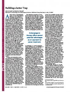
H Norm = 1000 ( H ( S ) / log 2 B ) . In other words, we use an integer in the 0..1000 range to represent the range between minimum and maximum entropy regardless of the value of B. It is not difficult to see that neighboring windows (that differ in their starting position by one) will have strongly correlated entropy estimates as their content differs by one byte. This allows for a very efficient incremental computation of estimates based on previous ones. Using a pre-computed (B+1) x (B+1) table of all the possible changes, we reduce the incremental computation to two increments, an addition and a table lookup. Next, we generated a set of histograms to illustrate the relationship between Hnorm and the different file types. For that purpose, we generated all the features of size B = 128 for all the files in the set. As Figure 1 clearly demonstrates, one can find a rather characteristic distribution for each type, and, in fact, a similar kind of entropy analysis has been proposed as a means of identifying data belonging to different file types. A few basic observations are worth mentioning: • The data covers the average case and individual objects, especially small ones, can and do deviate significantly from the average case. One simple example are composite types, such as doc/xls— the histogram on Figure 1a/g shows a significant concentration of high-entropy data due to embedded compressed images (~2/3 of all doc files contained at least one image). Evidently, a file which contains no compressed data would have a very different distribution. A small image will have, in relative terms, more low-entropy header data than the average, simply because the header is a larger fraction of overall file size.
3
0.18
0.35
0.16
0.30
0.14 0.25
Probability
Probability
0.12 0.10 0.08
0.20 0.15
0.06 0.10 0.04 0.05
0.02 0.00
0.00 0
100
200
300
400
500
600
700
800
900
1000
0
100
200
300
400
(a) H norm distribution: doc
500
600
700
800
900
1000
700
800
900
1000
700
800
900
1000
700
800
900
1000
(b) H norm distribution: gz 0.35
0.10 0.09
0.30
0.08 0.25
Probability
Probability
0.07 0.06 0.05 0.04
0.20 0.15 0.10
0.03 0.02
0.05
0.01 0.00
0.00 0
100
200
300
400
500
600
700
800
900
0
1000
100
200
300
400
500
600
(d) H norm distribution: jpg
(c) H norm distribution: html 0.25
0.12
0.10
0.20
Probability
Probability
0.08 0.15
0.10
0.06
0.04 0.05
0.02
0.00
0.00 0
100
200
300
400
500
600
700
800
900
0
1000
100
200
300
0.040
0.08
0.035
0.07
0.030
0.06
0.025
0.05
Probability
Probability
400
500
600
(f) H norm distribution: txt
(e) H norm distribution: pdf
0.020 0.015
0.04 0.03
0.010
0.02
0.005
0.01
0.000
0.00 0
100
200
300
400
500
600
(g) H norm distribution: xls
700
800
900
1000
0
100
200
300
400
500
600
(h) H norm distribution: xml
Figure 1 Empirical probability density functions for experimental data sets
4
•
•
•
All the text data types (html, txt, xml) have very similar distributions, which is a rather intuitive result. Nonetheless, we will see that there are non-trivial differences with respect to false positive rates. All of the compressed data types—gz, jpg, and pdf—exhibit a very compact bell at the high end of the spectrum. Jpg objects show a blip of lowentropy data due to header information and relatively small average size (~90KB). In contrast, gz objects do not—recall that each contains a single compressed file and, thus, has a minimal header. The pdf set is the only one the three that contains a notable amount of text (meta data) and that manifests itself as a smallish, broad peak around 700. The doc/xls files have the most varied distributions as they have complex internal structure (essentially, a small file system) and serve as containers for other object types, such as images. This results in peaks at both ends of the spectrum, along with multiple other local peaks reflecting large amounts of table and textual information.
In the following section we explore the relationship between the entropy measure of a feature and its false positive (FP) probability.
4. Entropy-based FP Prediction It is worth noting that the relationship between the entropy of a feature and its uniqueness is rather complex—a fact that appears to be underappreciated in the digital forensics literature. Occasionally, the entropy number tells pretty much the whole story: for the very low end of the spectrum, it basically means that the features are mostly the same repeat character with some small variations. Thus, we can be quite certain that this kind of data produces weak features that cannot be reliably attributed. Most of the time, however, the entropy measure does not tell us the whole story and should be treated only as a hint, especially when applied to short sequences. For example, assuming a B=64, any sequence containing 64 different characters would have maximum entropy. Yet, that is statistically unlikely so those are usually predictable features, such as tables, that are poor candidates for characteristic features. As the following data shows, things are not straightforward through the rest of the spectrum either. We begin our discussion with a focus on pure text (txt) data as it has the fewest artifacts related to formatting and can serve as a baseline for several
other types. After some experiments on network data, we decided to work with finer-grain features of 64 bytes so, unless otherwise noted, the data is for B=64. First, let us examine consider the relationship between Hnorm and the FP rate. In other words, we estimate empirically the conditional probability that a feature is non-unique, given a certain entropy number. The result is shown as a bar chart on Figure 2 (data has been aggregated by a factor of ten to allow for proper chart display). We can see that, for extremely low entropy scores, we get close to 100% false positives. That number drops sharply and, for scores of 200+, the probability stays below 10%, with numbers staying below 5% for most of that interval. To put these probabilities into perspective, consider the overall fraction of features have a particular entropy number. The line graph on Figure 2 gives the cumulative distribution of features as a function of the entropy measure Hnorm. By and large, it is good news—if we decide to drop from consideration all features with a measure below 200, for example, this would result in the elimination of only 2.21% of the features from consideration. If we moved the cut off point to 250—the first point where FP rate drops below 0.05, we would still keep 97% of the features. Yet, the figure shows that, to the right, the FP rate forms another little peak, which we may want to also exclude from consideration. Obviously, the lower we drop the FP threshold for inclusion, the lower the overall (unconditional) FP rate, and the larger the fraction of excluded features. To better understand this relationship, on Figure 2 we have shown the fraction of included features (coverage) as a function of the selected threshold for values from 0.1 to 0.01. The coverage stays almost constant for threshold FP rates down to 0.07, with the corresponding expected overall FP rate of about 0.035. As the threshold drop from 0.06 to 0.03, coverage drops from 0.80 to 0.47, with overall FP rate going from 0.025 to 0.011. Note that lower FP coverage is not all bad—it serves as a natural compression by reducing the number of features independently of other compression techniques that may be used, such as Bloom filters [1], [3]. If the search targets are large, reducing FP rate may well outweigh some imperfections in coverage. Below a threshold of 0.02, we see a catastrophic collapse as the selection scheme completely loses coverage.
5
1.00
1.00
FP Rate Data CDF
0.90
0.80
0.80
0.70
0.70
0.60
0.60
0.50
0.50
0.40
0.40
0.30
0.30
0.20
0.20
0.10
0.10
0.00
Data CDF
FP Rate
0.90
0.00 0
100
200
300
400
500
600
700
800
txt: H norm
Figure 2 FP rate and data CDF for plain text 1.00
FP Rate Coverage
Overall FP Rate
0.045
0.90
0.040
0.80
0.035
0.70
0.030
0.60
0.025
0.50
0.020
0.40
0.015
0.30
0.010
0.20
0.005
0.10
0.000
Feature Coverage
0.050
0.00 0.10
0.09
0.08
0.07
0.06
0.05
0.04
0.03
0.02
0.01
FP Threshold
Figure 3 Overall FP rate and feature coverage based on FP threshold
6
We also examined the distribution of the coverage for the threshold of 0.03 to understand how frequently big gaps in the coverage occur. Since the average distance between two selected features is only 1.59 we used the histogram on Figure 3 to better understand the behavior. It shows the cumulative probability that the gap in coverage falls within a particular interval. Inversely, we can infer the probability that it is greater than any particular number. For example, the probability that the gap exceeds 1024 bytes is 1 on 100,000. It is evident that, even when overall coverage drops in half, the local coverage stays largely even, although notable but infrequent gaps do occur. Having established a baseline with plain text, now consider the behavior of more complex data types, such as html. Generally, we would expect for html to be very similar given that it is designed to be human-readable; however, it is of interest to see the effects of common formatting on feature properties. As Figure 4 clearly shows, the effect on FP rates is quite dramatic. In particular, the FP rate never drops below 0.027, and, with the exception of very low entropy features, remains consistently higher than the corresponding ones for plain text. While this makes intuitive sense due to the fact that html formatting brings more predictability into the features, we have not seen such issues discussed in the evaluation of similarity schemes. We should emphasize that these results are very generic and, any similarity scheme that picks features at random—as all current ones effectively do—will see non-trivial differences in its FP rates depending on the underlying data.
5. Statistically Improbable Features We could, of course, reproduce more charts for the different file types; however, that would not answer the question of how to utilize the presented data for similarity discovery. One possibility is to use the per-type FP charts and pick features with the lowest FP rates. That would, in principle, produce the lowest average FP rates. However such features tend to be clustered—if we estimate (based on the entropy measure) that a feature will have a low FP, then the neighboring features will have a very similar, or identical entropy as they differ by one byte. Further, we would like a scheme that produces nice coverage without the need to calculate the hash of every single feature. Our basic idea is to use the observed distribution of the computed entropy estimates as the basis for selecting statistically improbable features. For that purpose, we associate a precedence rank with each
entropy measure value that is proportional to the probability that it will be encountered. In other words, the least likely feature as measured by its entropy score gets the lowest rank, whereas the most common one is assigned the highest. Assuming a fixed feature size of length B, we can associate precedence scores for all of the L-B features of an object, where L is the size of the object. Features eliminated due to too low/high score are assigned a special null score to prevent their selection altogether. Next, we pick a window size of W and, for every W consecutive rank scores, we select the leftmost minimum score (this is a sliding window type of calculation). All the while we keep count of how many times every feature has been picked as the minimum score. Thus, if a feature is picked k times (k ∈ [1..W]), it means that it is the local minimum within a window of size W + k – 1 and can be viewed as a measure of the relative local popularity of a particular feature. Finally, we pick a threshold parameter t and select all features with k ≥ t as the fingerprinting features of the object, and hash them using MD5. Figure 5 illustrates the process for a 320-byte snippet from a gz file (L = 320). For B = 64, we can generate 256 consecutive entropy estimates and 256 corresponding rank scores (top chart). Note that the entropy estimate changes minimally between neighboring estimates, and generally stays within a narrow range. However, every once in a while, it drifts out of that range, and the rank score drops sharply (around offsets 40 and 180 on the chart). This usually results in a popular feature, although a drop is not a necessary condition for high popularity (e.g. offset 120). Figure 5 also shows that for a threshold value of t = 16, four features would be selected from the snippet, whereas t = 48 results in two features being selected. There are two obvious questions that arise in a real implementation: Which distribution should we choose to base our rankings on? Is there enough local variability in entropy scores to support the heuristic that local choices will tend to pick the same features? In general, the first question is unlikely to have a single correct answer. A simple generic solution is to have a benchmark set and use it to set the ranks. This could be customized by profiling actual traffic for the specific deployment scenario. Yet, under any circumstances, we can expect that traffic will nontrivially deviate from our definition of typical so if our method is too sensitive to that choice, it would be less useful as it would result in fewer local agreements on the choice of features. To compensate, we would have to lower t to select enough features.
7
0.16 0.14 0.12
FP Rate
0.10 0.08 0.06 0.04 0.02 0.00 0
100
200
300
400
500
600
700
800
900
H norm
Figure 4 FP rate by entropy measure for HTML 1000 900
Rank Score
800 700 600 500 400 300 200 100 0
Offset
0
16
32
48
64
80
96
112
128
144
160
176
192
208
224
240
70
Popularity Score
60
t = 48
50
40
30
20
t = 16
10
Figure 5 Rank and popularity scores for a 320-byte snippet: L=320, B=64, W = 64 800
64-16
64-24
64-32
64-40
64-48
64-56
64-64
Common Features
700
600
500
400
300
200
100
0
5
15
25
35
45
55
65
75
85
95
Data Overlap (%)
Figure 6 Feature selection performance on random data
8
Therefore, we could choose the doc distribution as our reference point and use it on all the sets. Going back to Figure 1, we can see that it almost serves as a composite of the rest with several local peaks. Actual data will effectively mask out parts of the ranking— e.g. compressed data will have little use for entropy ranks to the left of its bell, whereas text data will not need anything to the right of its bell. The answer to the second question is a confident ‘yes’—even random data exhibits a bell-shaped distribution of entropy scores so even within a relatively small of window of 64-128 bytes, a few of the features are likely to stand out as statistically improbable, relative to the rest.
6. Measuring File Similarity We are now ready to go back to our original problem of finding similar objects. To establish a baseline measurement of the effectiveness of the described methods, we ran a controlled experiment using random data and known amounts of overlapping content. Specifically, we used two randomly generated files and produced mixed versions of them in the following fashion: take x percent of file #1 and mix with 100-x percent from file #2. The mixing was done in blocks of 512 bytes and we used 21 values for x: 0, 5, 10, …, 100. Note that we selected the blocks at random so even the 100% case is not an identical file but a file containing the same data block in a random permutation. Further, we fixed W = 64, and varied t from 16 to 64 with a step of 8. Figure 6 summarizes the results. As we can see from the chart, the number of common features increases linearly with the increase of the amount of data in common and the slope of the increase is determined by the threshold parameter t. Generally, a lower the value for t means that more features are retained, whereas a higher value selects fewer features and improves compression. In this case, t = 16 retains an average (over the different runs) of 847 features, whereas t = 64 only 110. Using an MD5 hash to compress the feature representation would mean that our storage requirements would be 13,552 and 7,040 bytes, respectively. This yields corresponding compression ratios of 3.8:1 and 7.2:1 that can be further improved 10 times by using a Bloom filter with 10 bits per element and 0.8% FP rate. Further reductions are possible by selecting a bigger value for W, such as 128, 256, 512. The above results can readily be replicated for compressed data types such as jpg, pdf, and gz. For text, the results are quite similar for unrelated text, however, things like style and common topic do tend
to yield higher results as the syntactic similarity increases. Generally, the results for non-random data need to be evaluated with respect a baseline FP rate, which is relatively straightforward to obtain from a representative set of files. Alternatively, one could use the set to generate a set of duplicate features and ignore them in the actual data. A large-scale experimental validation of an early prototype implementation on 4.6GB of real data (Table 1) is the subject of a separate paper. In summary, we were able to detect files within simulated network traffic based on a single packet with 0.9987 to 0.9844 accuracy (depending on file type) for feature size of 64 and threshold of 16. Our current implementation is capable of 100MB/s sustained throughput on a quad-core processor—this includes feature selection, feature hashing, and comparison with a reference set. We expect that an improved implementation would need no more than two cores to sustain that rate.
7. Conclusions In this paper, we presented a new approach to selecting syntactic features for similarity measurements. Our work makes the following contributions: • Through empirical data, we have shown that a basic entropy measure can provide a valuable guideline with respect to the uniqueness of a particular feature. • We have shown that different data types exhibit different behavior and that similarity measures can be tuned to keep a lid on overall false positive rate. • We proposed a new method for selecting characteristic features that does not rely on a Rabin scheme to be content-sensitive. Instead, we use an entropy measure and empirical distribution data to select statistically improbable features. • The new method is very stable and predictable with the respect to the coverage it produces, and, unlike previous work, can easily be tuned to the underlying data. In the immediate future we plan to full develop a practical, high-performance tool that can be used to correlate evidence on a large scale.
9
8. References [1] B. Bloom, “Space/Time Tradeoffs in Hash Coding with Allowable Errors,” Communications of the ACM, vol 13 no 7, pp. 422-426, 1970. [2] S. Brin, J. Davis, H. Garcia-Molina. “Copy detection mechanisms for digital documents”. In Proceedings of the ACM SIGMOD Annual Conference, San Francisco, CA, May 1995. [3] A. Broder, M. Mitzenmacher, “Network Applications of Bloom Filters: A Survey,” Internet Mathematics, vol 1 no 4, pp. 485-509, 2005. [4] A. Broder, S. Glassman, M. Manasse, and G. Zweig, “Syntactic Clustering of the Web”. In Proceedings of the 6th International World Wide Web Conference, pp. 393-404, 1997. [5] M. S. Charikar. “Similarity Estimation Techniques from Rounding Algorithms”. In Proceedings of the 34th Annual ACM Symposium on Theory of Computing, 2002. [6] C. Y. Cho, S. Y. Lee, C. P. Tan, and Y. T. Tan. “Network forensics on packet fingerprints. 21st IFIP Information Security Conference (SEC 2006), Karlstad, Sweden, 2006. [7] Henziger, M., “Finding Near-Duplicate Web Pages: A Large-Scale Evaluation of Algorithms”, In Proceedings of the 29th Annual International ACM SIGIR Conference on Research & Development on Information Retrieval, Seattle 2006. [8] R. Karp, M. Rabin. "Efficient randomized patternmatching algorithms". IBM Journal of Research and Development 31 (2), 249-260, 1987. [9] A. Kirsch, M. Mitzenmacher, “Distance-Sensitive Bloom Filters,” Proceedings of the Algorithms, Engineering, and Experiments Conference (ALENEX 2006). [10] J. Kornblum, “Identifying almost identical files using context triggered piecewise hashing”, Proceedings of the 6th Annual DFRWS, Aug 2006, Lafayette, IN. [11] U. Manber. Finding similar files in a large file system. In Proceedings of the USENIX Winter 1994 Technical Conference, pages 1-10, San Fransisco, CA, USA, 1994. [12] M. Mitzenmacher, “Compressed Bloom Filters”, IEEE/ACM Transactions on Networks, 10:5, pp. 613620, October 2002. [13] K. Monostori, R. Finkel, A. Zaslavsky, G. Hodasz, M. Pataki, “Comparison of Overlap Detection
Techniques”. In Proceedings of the 2002 International Conference on Computational Science, Amsterdam, The Netherlands, (I) pp 51-60, 2002. [14] M. Ponec, P, Giura, H. Brnnimann, J. Wein, “Highly Efficient Techniques for Network Forensics, In Proceedings of the 14th ACM Conference on Computer and Communications Security, 2007, Alexandria, Virginia. [15] H. Pucha, D. Andersen, M. Kaminsky“. Exploiting Similarity for Multi-Source Downloads using File Handprints”. In Proceedings of the Forth USENIX NSDI, Cambridge, MA. Apr, 2007. [16] M. O. Rabin. “Fingerprinting by random polynomials”. Technical report 15-81, Harvard University, 1981. [17] S. Rhea, K. Liang, and E. Brewer. Value-based web caching. In Proceedings of the Twelfth International World Wide Web Conference, May 2003. [18] V. Roussev, Y. Chen, T. Bourg, G. G. Richard III, “md5bloom: Forensic filesystem hashing revisited”, Proceedings of the 6th Annual DFRWS, Aug 2006, Lafayette, IN. [19] V. Roussev, G. Richard III and L. Marziale, "Multiresolution similarity hashing", Proceedings of the Seventh Digital Forensic Research Workshop, 2007. [20] K. Shanmugasundaram, H. Bronnimann, N. Memon, “Payload Attribution via Hierarchical Bloom Filters,” Proceedings of the ACM Symposium on Communication and Computer Security (CCS'04), 2004. [21] N. Shivakumar and H. Garcia-Molina. “SCAM: a copy detection mechanism for digital documents”. In Proceedings of the International Conference on Theory and Practice of Digital Libraries (June 1995). [22] N. Shivakumar, H. Garcia-Molina, “Building a scalable and accurate copy detection mechanism”. In Proceedings of the ACM Conference on Digital Libraries (March 1996), 160-168. [23] N. Shivakumar, H. Garcia-Molina. “Finding nearreplicas of documents on the web”. In Proceedings of the Workshop on Web Databases (March 1998), 204212. [24] S. Schleimer, D. S. Wilkerson, and A. Aiken. "Winnowing: local algorithms for document fingerprinting. In SIGMOD '03: Proceedings of the 2003 ACM SIGMOD international conference on management of data, pages 76-85, New York, NY, USA, 2003. ACM Press.
10