building construction progress monitoring using ... - ISPRS Annals

ISPRS Annals of the Photogrammetry, Remote Sensing and Spatial Information Sciences, Volume IV-2, 2018 ISPRS TC II Mid-term Symposium “Towards Photogrammetry 2020”, 4–7 June 2018, Riva del Garda, Italy

BUILDING CONSTRUCTION PROGRESS MONITORING USING UNMANNED AERIAL SYSTEM (UAS), LOW-COST PHOTOGRAMMETRY, AND GEOGRAPHIC INFORMATION SYSTEM (GIS) Jezekiel R. Bognota, Christian G. Candidoa, Ariel C. Blancoa,b, and Jore Rene Y. Montelibanoc of Geodetic Engineering, University of the Philippines Diliman, Quezon City 1101 - (jrbognot, cgcandido, and acblanco)@up.edu.ph bTraining Center for Applied Geodesy and Photogrammetry, University of the Philippines Diliman, Quezon City 1101 cRadar Aero Resources, Quezon City 1109

aDepartment

Commission II, WG II/10 KEY WORDS: Photogrammetry, Building Construction, Progress Monitoring, UAS ABSTRACT Monitoring the progress of building’s construction is critical in construction management. However, measuring the building construction’s progress are still manual, time consuming, error prone, and impose tedious process of analysis leading to delays, additional costings and effort. The main goal of this research is to develop a methodology for building construction progress monitoring based on 3D as-built model of the building from unmanned aerial system (UAS) images, 4D as-planned model (with construction schedule integrated) and, GIS analysis. Monitoring was done by capturing videos of the building with a camera-equipped UAS. Still images were extracted, filtered, bundle-adjusted, and 3D as-built model was generated using open source photogrammetric software. The as-planned model was generated from digitized CAD drawings using GIS. The 3D as-built model was aligned with the 4D asplanned model of building formed from extrusion of building elements, and integration of the construction’s planned schedule. The construction progress is visualized via color-coding the building elements in the 3D model. The developed methodology was conducted and applied from the data obtained from an actual construction site. Accuracy in detecting ‘built’ or ‘not built’ building elements ranges from 82-84% and precision of 50-72%. Quantified progress in terms of the number of building elements are 21.31% (November 2016), 26.84% (January 2017) and 44.19% (March 2017). The results can be used as an input for progress monitoring performance of construction projects and improving related decision-making process.

1. INTRODUCTION Construction project monitoring has been an important and essential factor for the success of large-scale construction projects. Despite the importance of construction project monitoring, the traditional manual monitoring is still the prevalent and dominant practice (Braun et al., 2014). The current monitoring process is time consuming, labour intensive, and error-prone. The output of traditional manual monitoring are progress reports, the quality of which is heavily dependent on the experience of field personnel conducting the monitoring. Due to this, progress reports tend to be bias towards the field personnel’s interpretation of construction progress (Golparvar-fard et al., 2015). Because of the limitations of the terrestrial camera, fixed orbit satellites, and manned aerial photography, rapid and accurate 3D modelling of building has been a challenging task. However, recent developments in technology specifically the Unmanned Aerial System (UAS) has improved the efficiency and accuracy of 3D building modelling (Feifei et al., 2012). While UAVs are a popular tool for 3D building modelling, their application in image-based progress monitoring has not been fully investigated (Golparver-fard et al., 2014). Combined with the developments in image processing and geographical information system (GIS), the use of UAVs for construction progress monitoring could be achieved. Nonetheless, construction progress monitoring is still a challenging task. Problems such as occlusion of building elements, scaffoldings, and temporary structures are still affecting the quality of as-built 3D models produced. In addition, many of the photogrammetric software are still unavailable for public use such as AgiSoft Photoscan and Pix4D.

In the last decades, developments in image processing techniques, image acquisition techniques, and GIS have increased. The wider availability of reality capturing technologies led to applications in construction progress monitoring. With the advancement in photogrammetry and computer vision, new construction management techniques have been applied in construction operations and processes. Current research in construction progress monitoring focuses on utilization of imagebased modelling techniques combined with Building Information Models for the creation of as-built 3D models. Golparvar-fard et al. (2014) were able to develop an automated progress monitoring using unordered daily construction photographs and IFC-based Building Information Models. The paper presented a new and automated approach for recognition of construction progress that utilizes structure-from-motion techniques, multiview stereo, and voxel coloring and labelling algorithm for the reconstruction of a dense as-built point cloud. Subsequently, an IFC-based BIM and the as-built scene is fused using a coregistration. A machinelearning algorithm built upon by Bayesian probabilistic model is then used to detect physical progress. Finally, the system was able to visualize the reconstructed elements using an augmented reality approach. Braun et al. (2014) used the same concept but different approach in construction progress monitoring. As-built point cloud model was generated from the combination of structure-from-motion approach and measurement of control points in the construction site. For the dense point cloud generation, an approach that is based on Rothermel et al. (2012) was used. Then for the as-built and as-planned comparison, the planes are split and rasterize into cell size r. Two states were defined to determine progress in

This contribution has been peer-reviewed. The double-blind peer-review was conducted on the basis of the full paper. https://doi.org/10.5194/isprs-annals-IV-2-41-2018 | © Authors 2018. CC BY 4.0 License.

41


construction. The first state is based on the visibility constraints which is used to determine the status of the building. It uses a ray casting and probabilistic occupancy grid mapping to determine the status of each raster cell. Three states could be inferred using this method: 1) free, 2) occupied, and 3) unknown. “Free” refers to raster cell that is not occupied by any as-built point clouds. On the other hand, “Occupied” means that raster cell is occupied by the as-built point clouds. Lastly, “unknown” refers to raster cells that are occluded. All building parts that are labelled as “occupied” are further analyzed to determine if it does really exist. The analysis is based on point-to-model distance which used three criteria to determine the status. The result of the study is promising, enabling the identification of the status of building parts. This paper describes a new method of monitoring construction progress based on unmanned aerial system (UAS), low-cost photogrammetry, and GIS. First, videos of the building are captured using a UAS. An as-built 3D model is then generated from these images using free and open-source photogrammetry software. Subsequently, as-planned 3D model is generated using CAD plans and GIS. This is then integrated with the as-built 3D model. At this stage, the construction progress monitoring is carried out in a GIS environment. Different tools and functionalities in a GIS environment were used to perform construction progress monitoring. Finally, a labelling process is conducted on the as-planned 3D model to visualize the result of the construction progress monitoring. The methodology is then validated by tracking the status of each building element using the video acquired from the UAS.

2.2 CAD Refinement In this study, only four (4) types of building elements were considered for the digitization: 1) beam; 2) column; 3) slab; and 4) wall. Other elements that were deemed unnecessary such as aluminium panel, fixtures, pipelines, and such were removed from the CAD plans. The resulting CAD plan models only consist of the specified building elements. 2.3 Digitization of CAD Models CAD plan models were imported to ArcScene Environment for extruding the building elements into three-dimensions. Extrusion of the building elements was done using an attribute describing the base-height and layer-height of each building element. The combination of the base-height and layer-height value gives the 2D CAD plan models its three-dimensional feature. After extrusion, the 3D as-planned model was converted into a multipatch feature which allows the storage of a vector data into 3D format. 2.4 Georeferencing As-planned 3D Model To georeferenced the as-planned 3D model created, the spatial adjustment tool in ArcGIS toolbox was used. The ground control points established from the GNSS field survey were used to define the coordinate system of the as-planned 3D model. After defining the GCPs for the as-planned 3D model, the affine transformation was used to shift and transform the as-planned 3D model. 3. GENERATION OF AS-BUILT 3D MODEL

2. GENERATION OF AS-PLANNED 3D MODEL The generation of As-planned 3D models (Figure 1) consists of five steps namely: 1) Data acquisition; 2) CAD refinement; 3) digitization of CAD floor models; 4) 3D model generation; and 5) georeferencing as-planned 3D model.

Photogrammetric processing was employed for the generation of the As-built 3D models at various stages of building construction. The entire workflow consists of four phases as shown in Figure 2: 1) Reconnaissance and flight planning; 2) data acquisition and pre-processing; 3) photogrammetric data processing including image matching and generation of point clouds and meshes; and 4) Georeferencing the as-built 3D models.

Figure 2. As-built 3D model generation schema 3.1 Reconnaissance and Flight Planning Figure 1. As-planned 3D model generation schema 2.1 Data Acquisition Architectural and structural plans of building was acquired from the JITS Corporation, Inc. These architectural and structural plans contain the blueprint of the whole building which will be later digitized into different components.

Reconnaissance was first conducted around the building to be modelled to determine the suitable flight path for the unmanned aerial vehicle (UAV), a DJI Phantom. The area was scanned for possible obstructions such as trees and infrastructures including utilities. The geometry of the building was considered for the extent and flight pattern of the UAV. Initially, video scanning for each face of the building was carried out with the UAV flying left to right and left to right at different flying height. However, this


42


was reckoned to be time-consuming especially for monitoring purpose. It was decided to utilize an intelligent flight mode called POI (Point of Interest) to set the flight pattern of the UAV. A radius of 50 meters from the estimated center of the building and altitudes of 45 and 30 meters were used during the data acquisition (Figure 3).

3.4 Data Processing Several free and open-source software were utilized for the generation of the as-built models. The output of image filtering and selection was used for the as-built 3D model generation of the building. The filtered images were imported to VisualSFM for sparse point cloud reconstruction. VisualSFM uses the scale invariant transform algorithm (SIFT) to detect matching features from two images automatically (Figure 5). These matching features are stored as database of keypoints. The number of keypoints that could be identified in the image is heavily dependent on the image texture and resolution.

Figure 3. Point of Interest flight mode for data acquisition 3.2 Data Acquisition UAV flights were conducted on 13 November 2016, 11 December 2016, 14 January 2017, 5 February 2017 and 5 March 2017. A video recording scheme was used to capture the building. This was done to ensure sufficient overlaps between the images that will be extracted from the video. The video has a resolution of 2704 x 1520 pixels and a frame rate of 30 frames/second. 3.3 Data Pre-processing After the video acquisition, images (JPG format) were then extracted using Blender. In this study, all frames were extracted from the videos; therefore, 30 images were extracted each second. This was done to maximize the use of raw data and choose the best possible images from the video. Extracted images were subjected to filtering and selection such that distorted images and blurred images were excluded (see Figure 4). Blurred images typically contain less edges or boundaries due to subdued gradients. The Canny Edge Detection algorithm, which utilizes contrasting color between pixels to determine boundaries, was applied on the extracted images. The Canny Edge Detection algorithm typically involves five steps namely: 1) smoothing, 2) finding gradients, 3) non-maximum suppression, 4) thresholding, and lastly, 5) edge tracking. Usually, blurred images have minimal gradients since there is no much change in the intensity of the image. The white pixels in the canny edge processed image indicates edges; therefore, blurred images could be detected if the ratio of the white pixel with the total number of pixels in the image is low. Images with a high ratio were then selected for processing. For every 30 frames, one image that has the highest ratio of white pixels to black pixels was chosen.

Figure 5. Image to image matching using SIFT algorithm Following the keypoint identification, bundle adjustment was used to estimate camera poses and extract sparse point cloud. After generating the sparse point cloud of the as-built 3D model, a densified point cloud was derived by using the multi-view reconstruction software CMPMVS. CMPMVS is a multi-view stereo algorithm for reconstruction that takes a set of image and camera parameters. The output of the SfM software is taken as input and the images from the SfM output are then decomposed into sets of image clusters. The clustered images are processed independently and in parallel. All the processed clusters are then combined for reconstruction. The outputs are meshes and textured meshes saved in .ply and .wrl file. 3.5 Georeferencing As-built 3D model The output textured mesh was then georeferenced using MeshLab. The ground control points established from the field survey were used as the reference points. Residual errors for each GCPs were determined. To produce the dense point cloud of the as-built 3D model, the textured mesh was first cleaned and refined to remove the unnecessary portions. Using MeshLab, the cleaned and refined textured mesh was saved as XYZ file. The XYZ file was then loaded and exported as LAS file in the CloudCompare software.

4. CONTRUCTION PROGRESS MONITORING USING GIS The methodology for construction progress monitoring using GIS consist of: 1) Point cloud extraction; 2) parameters establishment; 3) threshold calculation; 4) visualization; and 5) validation. 4.1 Point Cloud Extraction

Figure 4. Sample blurred image (upper), sun’s glare (lower)

The georeferenced as-built and as-planned 3D models were first aligned and integrated using ArcGIS. Integration of as-built and as-planned 3D models allows for the extraction of point clouds from the as-built 3D model. Using the Locate LAS Points by


43


Proximity tool in ArcGIS v. 10.4, point clouds were extracted based on its corresponding building element in the as-planned 3D model. A model builder was created to automate the process of point cloud extraction.

construction monitoring wherein red indicates ‘not built’ elements while green indicates ‘built’ elements.

4.2 Establishment of Parameters

Validation of the status of each building element was done using the video acquired using the UAV. Each building element in the as-planned 3D model was inspected in the video to determine its status. The contingency table is used to report the number of true positives, false positives, false negatives, and true negatives (Table 1). Different performance metrics were then calculated using the contingency table (Table 2).

4.2.1 Point Cloud Density Computation: The number of points that falls within the proximity of a building element were determined and divided by the total surface area of the building element to get the point cloud density.

Point Cloud Density =

No.of points

(1)

total surface area

4.2.2 Difference in Centroid Computation: The difference in the computed centroid of the building element with the corresponding point clouds was calculated. Using the calculate geometry function, the centroid of each building element and its corresponding point clouds was determined. The centroids were then subtracted to get the difference in centroid locations.

Prediction n = total

Actual

After extracting the point clouds in the as-built 3D model, the following parameters were established for the determination of building element status: 1) Point cloud density computation; and 2) difference in centroid computation.

4.5 Validation

Built

Not built

Built

TP

FN

Not built

FP

TN

Table 1. Contingency table for the proposed methodology

4.3 Threshold Calculation The computed values of the point cloud density and difference in centroid were subjected to statistical analysis for threshold calculation. A simple graphical technique was first employed for removing outliers in the dataset. After removing the outliers in the dataset, a histogram was constructed for each type of building element and its underlying distribution was inspected (Figure 6). Simple quantitative statistics such as mean and standard deviation were employed for threshold calculation. The determined thresholds were then applied to separate the ‘built’ elements from ‘not built’ elements. Point Cloud Density Histogram (Wall)

Table 2. Different performance metrics used for the evaluation of methodology

0.03 0.025

5. RESULTS AND DISCUSSION

0.02

5.1 Generated As-built 3D Model

0.015 0.01 0.005 0 0

100

200

300

400

500

Figure 6. Sample histogram of point cloud density for a wall The building elements that satisfy the threshold were labelled as one (1) and considered as ‘built’ while building elements that did not satisfy the threshold were labelled as zero (0) and considered as not built. Linear regression was done to check if threshold yields better R-squared. 4.4 Visualization Visualization of the construction progress monitoring was done using ArcScene. A color-coding scheme was used to visualize the

In this study, five (5) as-built 3D models were generated. In regular time intervals for the duration of five (5) months, the UP College of Architecture (UPCA) building was captured by means of UAV. The first dataset (Nov. 13, 2016) was about 783 images processed in one day and thirteen hours. The second dataset (Dec. 11, 2016) was about 748 images processed in one day and fifteen hours. The third dataset (Jan. 14, 2017) was about 651 images with a total processing time of two days and seven hours. The fourth dataset (Feb. 05, 2017) was about 391 images with a total processing time of one day and seven hours. Lastly, the fifth dataset (Mar. 05, 2017) was about 748 images with a total processing time of one day and fourteen hours. Figure 7 shows a sample generated textured mesh. The textured meshes were then cleaned and refined to remove unnecessary data. The cleaned and refined textured meshes were converted to point clouds which were saved into LAS format (Figure 8).


44


graphical techniques, descriptive statistics, and linear regression, the optimum thresholds for each type of building element were identified. Table 3 shows the summary of the threshold calculation for each type of building element.

Flight Observations

Building Elem. Type

Point Cloud Density Threshold

Diff. in Centroid Threshold

Adjusted R2

Beam

11.796

0.753

0.573

Column

11.946

0.27

0.570

Slab

25.154

1.021

0.460

Wall

63.256

0.778

0.336

Beam

9.723

0.834

0.664

Column

3.634

0.365

0.601

Slab

25.493

1.391

0.646

Wall

29.672

0.502

0.382

Beam

8.73

0.908

0.690

Column

7.168

0.396

0.747

Slab

29.27

2.812

0.791

Wall

37.00

0.416

0.559

Nov. 13, 2016

Figure 7. Generated raw mesh for March 5,2017 flight observation

Jan. 14, 2017

Mar. 05, 2017

Table 3. Summary of threshold value for each type of building element

Figure 8. Processed LAS files for flight observations Mar. 05, 2017 5.2 Generation of As-Planned 3D Model The as-planned 3D model of the UPCA (Figure 9) was generated through (1) digitization of 2D CAD models and (2) alignment and integration of the as-planned and as-built 3D models.

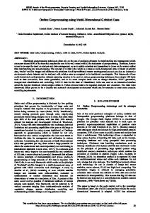
From the table, it can be observed that there is an increasing trend in the calculated R2. The calculated R2 for Mar. 05, 2017 are relatively higher compared to the R2 calculated from other flight observations. This indicates that the methodology succeeded in detecting building elements for Mar. 05, 2017 flight observation than the other flight observations. Analysing and observing the as-built 3D model derived for Mar. 05, 2017, there are less occlusions due to temporary objects such as scaffoldings, formworks, site fences, and other unnecessary materials that block or cover building elements. 2500 2000 1500 1000 500 0

2094

1813 1358 1095

528

665

November 13, 2016

January 14, 2017

Built

March 5, 2017

Not Built

Figure 10. Detected number of building elements using the methodology Figure 9. Isometric View of the As-Planned Model of UPCA (walls - yellow, columns - red, beams - green, slab/floor – gray). For the alignment of the as-planned and as-built 3D models, both were georeferenced using GCPs established from the horizontal control survey. A total of seven (7) GCPs were established to georeference both the as-planned and as-built 3D models. Each of the as-built 3D models were georeferenced separately. 5.3 Construction Monitoring Using GIS After the alignment of as-planned and as-built 3D models, point clouds were extracted from the as-built 3D models. The extracted point clouds were compared to its corresponding building elements in the as-planned 3D model to obtain the information for the parameter establishment. Thresholds were then calculated to separate ‘built’ and ‘not built’ building elements. Using simple

The total number of building elements presented in Figure 10 accounts for the total number of exterior and interior building elements. In most cases, interior building elements were labelled as ‘not built’ which can mainly be ascribed to three reasons: (1) the acquisition geometry does not allow interior building elements to be seen or captured by the video, (2) occlusions due to other objects which have already been built, (3) and missing illumination for the interior elements in the building (Tuttas, Braun, Borrman, & Stilla, 2015). For the exterior building elements that were occluded by other building elements, it was observed that they were also partially reconstructed by the algorithm resulting to non-detection of the building element. This added to the low accuracy and precision of the results.


45


Using the number of building elements detected using the methodology, in terms of exterior elements, the quantified progress of the building for November 13, 2016 is 21.31%. For January 14, 2017, the quantified progress of the building is 26.84% and lastly, for March 05, 2017, the quantified progress of the building is 44.19%. 5.4 Validation Results The accuracy and reliability of the methodology is analysed using a binary contingency table and different performance metrics. The predicted status of each building elements was tabulated and compared to its actual status in a dichotomous contingency table. For Nov. 13, 2016, 2,478 building elements were classified. The following legends are used for the succeeding tables: TP - Hit rate, FP - False Alarm Rate, and FN - Miss Rate.

Table 6. Accuracy assessment for Mar. 05, 2017 The result showed that the building elements could be detected using the available GIS tools. An accuracy of 82 – 84% and a precision of 50 – 72% were achieved by the methodology.

5.5 Visualization of Construction Progress Monitoring For the predicted status, each of the building elements that satisfied the thresholds were classified as ‘built’ while building elements that did not satisfy the threshold were classified as ‘not built’. Figure 10 shows sample visualization of predicted status of the building on March 5,2017.

Table 4. Accuracy assessment for the case of Nov. 13, 2016 The methodology registered an accuracy of 84.42% and precision of 49.81%. Although the methodology had a fair accuracy, the registered precision is lower than 50% which could be attributed to the presence of temporary objects such as scaffoldings and formworks in front of building elements. Other possible causes of low precision for Nov. 13, 2016 result are (1) nonrepresentation of a building element which resulted to poor reconstruction, and (2) occlusions which resulted to partial reconstruction. The TP rate was calculated to be 68.49%, the FP rate to be 12.66% and FN Rate to be 31.51%. For Jan. 14, 2017, the methodology was found to have 82.32% accuracy while having precision of 60.50%. The TP rate was found to be 73.85%, the FP rate was 15.03 % and the FN rate was 26.15%.

Table 5. Accuracy assessment for Jan. 14, 2017 For March 5, 2017, the methodology registered an accuracy of 84.10% while having the precision of 72.55%. It is noticeable that there is an improvement in the precision of the methodology as the observation goes by. This can be attributed to better reconstruction of the model since it could be observed that a lot of temporary objects such as scaffoldings and formworks were already removed from the building. The calculated TP rate of the methodology was 79.27%, while the FP rate and FN rate were found to be 13.70% and 20.72% respectively.

B Built u Not Built i l Predicted Status Isometric View Figure 10. March 5, 2017 t

6. CONCLUSION AND RECOMMENDATIONS This paper presented a methodology for construction progress monitoring that is based on Unmanned Aerial System (UAS), low-cost photogrammetry, and Geographic Information System (GIS). Images extracted from the UAS videos generated an asbuilt dense point cloud models which were later used for construction progress monitoring. Subsequently, the as-planned 3D model of the UPCA building was produced by digitization of the CAD plans, specifically the structural and architectural plans in ArcGIS. After which, alignment of as-planned and as-built models was done using the same platform. For the determination of the construction progress, GIS tools and functionalities were utilized. Point clouds were first extracted from the as-built 3D models and compared to the corresponding building elements in the as-planned 3D model using the parameters established. Thresholds were calculated from the parameters to separate the built building elements from the notbuilt or unverified building elements. Using the video for validation, the methodology for construction progress monitoring yielded satisfactory results. The methodology did well in detecting building elements having an accuracy of 82 - 84 % and a precision of 50 - 72%. Based on the results, the quantified progress in terms of the number of building elements are 21.31% for November 2016, 26.84% for January 2017, and 44.19% for March 2017.


46


Finally, visualization of the result of the methodology was done in 3D using ArcGIS. Animations were created from the result of methodology to better visualize the construction phases. Future research on techniques regarding 3D reconstruction of images is recommended since the quality of as-built 3D model relies heavily on the process of reconstruction. More experiments the acquisition of images should be conducted. Also, the methodology for construction progress monitoring needs to be further enhanced by automating the entire process of monitoring. This will lessen if not eliminate the dependence on the user leading to improved efficiency and accuracy. Furthermore, it is also recommended to apply the methodology in the beginning of the construction phase since this will better represent the status of building elements as the occluded and not visible building elements will be captured by the UAV. Lastly, it is suggested to conduct further research on methods regarding the removal of scaffoldings, temporary walls, formworks, and other unnecessary materials that affect the detection of building elements.

8. ACKNOWLEDGEMENTS The authors thank Engr. Allen and Arch. Jester of JITS Construction Corporation, Inc. for their support and guidance during the field surveys at the construction site. To the EnviSAGE Research Laboratory for generosity, kind considerations, and use of workstations and GPS receivers. Lastly, the authors thank Engr. Rey Rusty Quides and Engr. Ian Estacio for the technical support. Dissemination of this study is supported by the Philippines’ Department of Science and Technology – Science Education Institute (DOST-SEI) Engineering Research and Development for Technology (ERDT) Program.

REFERENCES Braun, A., Tuttas, S., Borrmann, A., & Stilla, U., 2014. A concept for automated construction progress monitoring using BIMbased geometric constraints and photogrammetric point clouds. Journal of Information Technology in Construction (ITcon), Special Issue: ECPPM 2014, (20) 68-79. Braun, A., Tuttas, S., Borrmann, A., & Stilla, U., 2015. Validation of BIM components by photogrammetric point clouds for construction site monitoring. ISPRS Annals of the Photogrammetry, Remote Sensing and Spatial Information Sciences, Vol. II-3/W4, 231 – 237 Golparvar-Fard, Forsyth, D., & Karsch, K., n.d. ConstructAide: analyzing and visualizing construction sites through photographs and building models. ACM Transactions on Graphics (TOG) – Proceedings of ACM SIGGRAPH Asia 2014, 33(6)

UAVs for automated construction progress monitoring. 2015 International Workshop on Computing in Civil Engineering McCulloch, B., 1997. Automating Field Data Collection in Construction Organizations. In Construction Congress V: Managing Engineered Construction in Expanding Global Markets. ASCE, pp. 957-963. Naik, G., Aditya, M., & Naik, S., 2011. Integrated 4D model development for planning and scheduling of a construction project using geographical information system. 2nd International Conference on Construction and Project Management IPEDR, (15). Navon, R., 2005. Automated Project Performance Control of Construction Projects. Automation in Construction, 14(4), pp. 467-476. Pazhoohesh, M., Shahmir, R., Zhang, C., 2015. Investigating Thermal Comfort and Occupants Position Impacts on Building Sustainability Using CFD and BIM. 49th International Conference of the Architectural Science Association 2015. pp. 257-266. Qu, T., Zang, W., Peng, Z., Liu, J., Li, W., Zhu, Zhang, B., & Wang, Y., 2017. Construction site monitoring using UAV oblique photogrammetry and BIM technologies. Protocols, Flows, and Glitches, Proceedings of the 22nd International Conference of the Association for Computer-Aided Architectural Design Research in Asia (CAADRIA). Remondino, F., & El-Hakim, S., 2006. Image-based 3D modelling; a review. The Photogrammetric Record, (115) 269291 Saidi, K., Lytle, A. M., Stone, W. C., 2003. Report of the NIST Workshop on Data Exchange Standards at the Construction Job Site. InProc., ISARC-20th Int. Symp. On Automation and Robotics in Construction. pp. 617-622. Son, H., Kim, C., 2010. 3D Structural Component Recognition and Modelling Method Using Color and 3D Data for Construction Progress Monitoring. Automation in Construction. 19(7), pp. 844-854. Wu, C., 2013. Towards Linear-Time Incremental Structure from Motion. 2013 International Conference on 3D Vision, Seattle, Wash., 405-426. http://ccwu.me/vsfm/vsfm.pdf. [Accessed: 31st January 2017] Zhang, X., Bakis, N., Lukins, T. C., Ibrahim, Y. M., Wu, S., Kagioglou, M., Trucco, E., 2009. Automating Progress Measurement of Construction Projects. Automation in Construction, (18) 294-301.

Golparvar-Fard, M., Pena-Mora, F., Alboleda, C., Lee, S., 2009 Visualization of Construction Progress Monitoring with 4D simulation Model Overlaid on Time-Lapsed Photographs. Journal of Computing in Civil Engineering, (23) 391-404. Golparvar-Fard, M., Pena-Mora, & F., Savarese, S., 2014. Automated progress monitoring using unordered daily site photographs and IFC-based building information models. Journal of Computing in Civil Engineering, (29) Golparvar-Fard, M., Han, K., & Lin, J., 2015. A framework for model-driven acquisition and analytics of visual data using


47