www.itcon.org - Journal of Information Technology in Construction - ISSN 1874-4753
A CONCEPT FOR AUTOMATED CONSTRUCTION PROGRESS MONITORING USING BIM-BASED GEOMETRIC CONSTRAINTS AND PHOTOGRAMMETRIC POINT CLOUDS SUBMITTED: November 2014 REVISED: December 2014 PUBLISHED: January 2015 at http://www.itcon.org/2015/5 GUEST EDITORS: Mahdavi A. & Martens B. Alexander Braun Chair of Computational Modelling and Simulation;
[email protected] Sebastian Tuttas Department of Photogrammetry and Remote Sensing;
[email protected] Andre Borrmann Chair of Computational Modelling and Simulation;
[email protected] Uwe Stilla Department of Photogrammetry and Remote Sensing;
[email protected]
SUMMARY: On-site progress monitoring is essential for keeping track of the ongoing work on construction sites. Currently, this task is a manual, time-consuming activity. The research presented here, describes a concept for an automated comparison of the actual state of construction with the planned state for the early detection of deviations in the construction process. The actual state of the construction site is detected by photogrammetric surveys. From these recordings, dense point clouds are generated by the fusion of disparity maps created with semi-global-matching (SGM). These are matched against the target state provided by a 4D Building Information Model (BIM). For matching the point cloud and the BIM, the distances between individual points of the cloud and a component’s surface are aggregated using a regular cell grid. For each cell, the degree of coverage is determined. Based on this, a confidence value is computed which serves as basis for the existence decision concerning the respective component. Additionally, process- and dependency-relations are included to further enhance the detection process. Experimental results from a real-world case study are presented and discussed. KEYWORDS: progress monitoring, point clouds, as-built as-planned comparison REFERENCE: Alexander Braun, Sebastian Tuttas, Andre Borrmann, Uwe Stilla (2015). A concept for automated construction progress monitoring using BIM-based geometric constraints and photogrammetric point clouds. Journal of Information Technology in Construction (ITcon), Special Issue: ECPPM 2014, Vol. 20, pg. 68-79, http://www.itcon.org/2015/5 COPYRIGHT: © 2015 The authors. This is an open access article distributed under the terms of the Creative Commons Attribution 3.0 unported (http://creativecommons.org/licenses/by/3.0/), which permits unrestricted use, distribution, and reproduction in any medium, provided the original work is properly cited.
ITcon Vol. 20 (2015), Braun et al., pg. 68
1. INTRODUCTION The traditional, manual construction progress assessment with human presence is still dominating. The main reason is the lack of reliable and easy to use software and hardware for the demanding circumstances on construction sites. Automating construction progress monitoring promises to increase the efficiency and precision of this process. It includes the acquisition of the current state of construction, the comparison of the actual with the target state, and the detection of variations in the schedule and/or deviations in the geometry. A Building Information Model (BIM) provides a very suitable basis for automated construction progress monitoring. A BIM is a comprehensive digital representation of a building comprising not only the 3D geometry of all its components but also a semantic description of the component types and their relationships (Eastman 1999; Eastman et al., 2011). The model is intended to hold all relevant information for all project participants. In addition to the description of the building itself, it also comprises process information, element quantities and costs. A Building Information Model is a rich source of information for performing automated progress monitoring. It describes the as-planned building shape in terms of 3D geometry and combines it with the as-planned construction schedule. The resulting 4D model (Webb et al., 2004) combines all relevant information for the complete construction process. Accordingly, the planned state at any given point in time can be derived and compared with the actual construction state. Any process deviation can be detected by identifying missing or additional building components. For capturing the actual state of the construction project, different methods can be applied, among them laser scanning and photogrammetric methods. With both point clouds can be generated that hold the coordinates of points on the surface of the building parts but also of many different temporary objects which are not modelled in the BIM. The main steps of the proposed monitoring approach are depicted in Fig. 1. The minimum information, which has to be provided by the BIM, is a 3D building model and the process information (construction start and end date) for all building elements. From this, the target state at a certain time step t is extracted. Subsequently the target state is compared to the actual state, which is captured by photogrammetric techniques in this study. Finally, the recognized deviations are used to update the schedule of the remaining construction process.
Figure 1: Construction progress monitoring schema The paper is organized as follows: Section 2 gives an overview on related work in the field. The proposed progress monitoring procedure is explained in detail in Section 3 and first experimental results are presented in Section 4. The paper concludes with a summary and discussion of future work.
ITcon Vol. 20 (2015), Braun et al., pg. 69
2. RELATED WORK 2.1 Monitoring and object verification Mainly as-built point clouds can be acquired by laser scanning or imaged-based/photogrammetric methods. In Boschè and Haas (2008) and Boschè (2010) a system for as-built as-planned comparison based on laser scanning data is presented. The generated point clouds are co-registered with the model with an adapted Iterative-Closest– Point-Algorithm (ICP). Within this system, the as-planned model is converted to a point cloud by simulating the points using the known positions of the laser scanner. For verification, they use the percentage of simulated points, which can be verified by the real laser scan. Turkan et al. (2012), Turkan et al. (2013) and Turkan et al. (2014) use and extend this system for progress tracking using schedule information, for estimating the progress in terms of earned value and for detection of secondary objects, respectively. Kim et al. (2013a) detect specific component types using a supervised classification based on Lalonde features derived from the as-built point cloud. An object is regarded as detected if the type derived from the classification is the same as in the model. As above, the model also has to be sampled into a point representation here. Zhang and Arditi (2013) introduce a measure for deciding four cases (object not in place (i), point cloud represents a full object (ii) or a partially completed object (iii) or a different object(iv)) based on the relationship of points within the boundaries of the object and the boundaries of shrunk object. The authors test their approach in a very simplified test environment, which does not include any problems, which occur on data acquired on a real construction site. The usage of cameras as acquisition device comes with the disadvantage of a lower geometric accuracy compared to the laser scanning point clouds. However, cameras have the advantage that they can be used more flexible and their costs are much lower. Because of the reasons mentioned above there is the need for other processing strategies if image data instead of laser scanning date is used. Rankohi and Waugh (2014) give an overview and comparison of image-based approaches for the monitoring of construction progress. Ibrahim et al. (2009) use a single camera approach and compare images taken over a certain period and rasterize them. The change between two timeframes is detected through a spatial-temporal derivative filter. This approach is not directly bound to the geometry of a BIM and therefore cannot identify additional construction elements on site. Kim et al. (2013b) use a fixed camera and image processing techniques for the detection of new construction elements and the update of the construction schedule. Since many fixed cameras would be necessary to cover a whole construction site, more approaches rely on images from hand-held cameras covering the whole construction site as in our and the approaches in the following. For the scale of the point cloud, stereo-camera systems can be used, as done in (Son and Kim, 2010), (Brilakis et al., 2011) or (Fathi and Brilakis 2011). Rashidi et al. (2014) propose to use a coloured cube with known size as target, which can be automatically measured to determine the scale. In our approach the scale is introduced using known coordinates in the construction site coordinate system. In Goldpavar-Fard et al. (2011a) image-based approaches are compared with laser-scanning results. The artificial test data is strongly simplified and the real data experiments are limited to a very small part of a construction site. Only relative accuracy measures are given since no scale was introduced to the photogrammetry measurements. Golparvar-Fard et al. (2011b) and Golparvar-Fard et al. (2012) use unstructured images of a construction site to create a point cloud. The orientation of the images is performed using a Structure-from-Motion process (SFM). Subsequently, dense point clouds are calculated. For the comparison of as-planned and as-built, the scene is discretized into a voxel grid. The construction progress is determined in a probabilistic approach, in which the thresholds for detection are determined by supervised learning. In this framework, occlusions are taken into account. This approach relies on the discretization of the space by the voxel grid, having a size of a few centimeter. In contrast to this, the deviation of point cloud and building model are calculated directly in our approach and we introduce a scoring function for the verification process. In contrast to most of the discussed publications, we present a test site which presents extra challenges for progress monitoring due to the existence of a large number of disturbing objects, such as scaffolding.
2.2 Process information and dependencies Process planning is often executed independently from conceptual and structural design phases. Current research follows the concept of automation in the area of construction scheduling.
ITcon Vol. 20 (2015), Braun et al., pg. 70
Tauscher describes a method that allows a partly automated generation of the scheduling process (Tauscher, 2011). He chooses an object-oriented approach to categorize each component according to its properties. Accordingly, each component is assigned to a process. Subsequently, important properties of components are compared with a process database to group them accordingly into relating process categories and assign the corresponding tasks to each object. Suitable properties for the detection of similarities are for example the element thickness or the construction material. With this method, a "semi - intelligent" support for process planning is implemented. Huhnt (2005) introduced a mathematical formalism that is based on the quantity theory for the determination of technological dependencies as a basis for automated construction progress scheduling. Enge (2009) introduced a branch and bound algorithm to determine optimal decompositions of planning and construction processes into design information and process information. These innovative approaches to process modelling form a very good basis for the automated construction monitoring, but have so far not been applied in this context and will be integrated into the concept presented here.
3. CONCEPT The developed methodology comprises the following phases: The building model and the process schedule is modelled and combined in a 4D model in the design and planning phase. During construction, the site is continuously monitored by capturing images of the as-built state. These are processed to create point clouds (Section 3.1), which are compared to the as-planned building model (as-built – as-planned comparison), what is described in Section 3.3. Process and spatial information can help to further improve the detection algorithms (Section 3.2).
3.1 Generation of as-built data The generation of the point cloud consists of four steps: Data acquisition (I), orientation of the images (II), image matching (III) and co-registration (IV). (I) Image acquisition: Photogrammetric imaging with a single off-the-shelf camera is chosen as data acquisition since it is inexpensive, easy to use and flexible. When using a camera, some acquisition positions such as on top of a crane can be reached more easily than when using a laser scanner. In addition, a major requirement is that the image acquisition process shall be conducted without any disturbance of the construction process. For performing a suitable acquisition, the construction site should be covered as complete as possible with overlapping images. For robustness and geometric accuracy each point which shall be reconstructed should be visible in at least three images. (II) Orientation: The orientation process is performed using the structure-from-motion system VisualSfM (Wu 2013) for an automatic generation of tie points. By means of the algorithm, also the relative orientations of the cameras are determined. For the following reasons we also introduce (manually) located control points: -
-
Having two control points, a distance is introduced and the missing scale is known then. With the help of control points, we can combine image groups that could not be orientated relatively to each other by the usage of only the automated measured correspondences. Reasons for separated image groups are e.g. non accessible positions which would be necessary for the acquisition of overlapping images. Control points are preferably in the same coordinates system as the one that is used for the construction work itself. If this is ensured, the point cloud is already co-registered to the model (assuming it is having also the same coordinate system).
The joint usage of control points and tie points is depicted in Fig. 2. The red circles are control points on stable points outside the construction site. The yellow lines represent the tie points based on autmatically detected features which connect overlapping images of one time step. Depending on the scene content the number of tie points connecting two images is much higher (tens to hundreds) than it is indicated by the four yellow lines in the figure.
ITcon Vol. 20 (2015), Braun et al., pg. 71
Figure 2: Image orientation process using control points and tie points Finally, a bundle block adjustment is accomplished to determine the exterior orientation of all images and the corresponding standard deviations. (III) Image matching: Using either calibrated parameters or parameters from self-calibration (i.e. determined simultaneously with the orientation parameter), distortion free images are calculated. In this study, a calibration device has been used to calibrate the camera in advance. As next step, stereo pairs (= image pairs which are appropriate for image matching, i.e. they shall be overlapping and shall have approximately an equal viewing direction) have to be determined. This done based on conditions on the baseline length and the angles between baseline and the camera axes. Every image of each stereo pair is rectified. That means that artificial camera orientations are calculated in such way that the camera axes of the pair are orientated normal to the base and parallel to each other. The rectified images are resampled from the original images. These images can then be used for dense-matching. For every pixel, a corresponding pixel in the other image is searched and the disparity is determined. The disparity is the distance of two pixels along an image row. To determine this, semi-global-matching (SGM) has been established in the last years (Hirschmüller 2008). Different implementations are available, e.g. SGBM in the openCV-library or LibTSGM (Rothermel et al. 2012), which is used here. By means of the disparity (what corresponds to the depth of the point) and the exterior orientations of both images, the 3D point can be triangulated for each pixel. To get a more robust estimation of the points, to reduce clutter and to estimate the accuracy of the depth, not simply all 3D-points of all stereo-pairs are combined but overlapping disparity maps are merged and only 3Dpoints are triangulated which are seen in at least three images. The following procedure follows the approach of Rothermel et al. (2012). First, an image has to be selected to become a master image. For every pixel of the undistorted master image, the disparities are interpolated from all k disparity maps the master image is involved in. Now for every pixel, k disparity values are available. An interval for the distance D from the camera centre to the 3D-point is determined by adding/subtracting an uncertainty value s from the disparity value. For every pixel, the depth values are clustered into one group if the intervals are overlapping. For calculating the final depth, the cluster having the most entries is chosen. The final value for D and its accuracy are determined by a least-square adjustment as described by Rothermel et al. (2012). The final 3D-point coordinates (X, Y, Z) are then calculated by X Y Z
T R n D
X0 Y0 Z 0
with rotation matrix R (from object to camera coordinate system), unit vector n from perspective centre to pixel and camera position X0, Y0, Z0. By applying the law of error propagation, the accuracy of the coordinates are calculated, using the standard deviations estimated in the bundle block adjustment (for R and X0, Y0, Z0) and in the determination of the depth (D), respectively. As last step, the point clouds of all master images are fused. For every point, the coordinate, the RGB-colour, the accuracy in depth, the accuracy for the co-ordinates and the ID of the reference image are stored. With the latter information, the ray from the camera to the point can be retrieved. This is a valuable information to apply visibility constraints for comparing the as-planned and as-built state. (IV) Co-registration: If the model coordinates as well as the control point coordinates are in a common construction site reference frame, a co-registration is not necessary. Otherwise, corresponding features that can be determined unambiguously in the model and the images have to be measured to calculate the transformation
ITcon Vol. 20 (2015), Braun et al., pg. 72
parameters. Of course, only building parts that have been proofed to be built correctly can be used for that. This has to be per-formed only once in an early time step, since the parameters are constant during the construction process.
3.2 Process information and technological dependencies In principle, a building information model can contain, besides geometry and material information, all corresponding process data for a building. The open source standard file format for storing building information models and related information is called Industry Foundation Classes (IFC). This file format is maintained and developed by the BuildingSMART organisation. In Version 4 of the IFC data model, the IfcTask entity was extended by the subtype IfcTaskTime to represent all process information and dependencies for a building element with direct relations to corresponding elements (BuildingSmart 2014). The IfcTask entity holds all task related information like the description, construction status or work method. The IfcTask is related to an object using IfcRelAssignsToProduct but could also be assigned to another relating process. The complete time-related information is hold in the sub entity IfcTaskTime. The information hold here include, next to the process duration, additional process data like EarlyStart or EarlyFinish. Therefore, this entity gives the possibility to combine geometry and process data with all monitoring related process information in a convenient way in one file. 3.2.1 Technological dependencies In current industry practice, construction schedules are created manually in a laborious, time-consuming and error-prone process. As introduced by Huhnt (2005), the process generation can be supported by detecting technological dependencies automatically. These dependencies are the most important conditions in construction planning. In the following, the concept of the technological dependencies is illustrated with the help of a simple two-storey building (Fig. 3).
Figure 3: Sample building used to illustrate technological dependencies The specimen building has four walls and a slab for each floor. One example for deriving dependencies from the model is the following: The walls on the second floor cannot be built before the slab on top of the first floor is finished. The same applies for this slab and the walls beneath it. These dependencies are defined as technological dependencies. Other dependencies that have to be taken into account for scheduling, such as logistical dependencies, are defined by process planners and thus cannot be detected automatically. A suitable solution for representing and processing these dependencies are graphs (Enge 2009). Each node represents a building element while the edges represent the dependencies. The graph is directed since the dependencies apply in one way. By convention, we define the edges as being directed from an object (predecessor) to the depending object (successor). Fig. 4 shows the technological dependencies of the sample building in the corresponding precedence relationship graph.
ITcon Vol. 20 (2015), Braun et al., pg. 73
Figure 4: The technological dependencies for the sample building depicted in Fig. 3 in a precedence relationship graph 3.2.2 Checkpoint Components The graph visualizes the dependencies and shows that all following walls are depending on the slab beneath them. In this research, these objects are denoted as checkpoint components. They play a crucial role for helping to identify objects from the point clouds that cannot be confirmed with a sufficient measure by the as built point cloud (see Section 3.3). In graph theory, a node is called articulation point, if removing it would disconnect the graph (Deo 2011). As defined in this paper, all articulation points represent a checkpoint component. An articulation point is an important feature for supporting object detection, since it depends on all its preceding nodes. In other words, all objects have to be finished before the element linked to the articulation point can be started to be built. As soon as a checkpoint component is detected (represented by an articulation point in the graph), all preceding nodes can be marked as completed. Doing so, also occluded objects can be detected by the proposed method.
3.3 Comparing as-built and as-planned state The as-planned – as-built comparison can be divided into several stages. This includes the direct verification of building components based on the point cloud (3.3.1) and the indirect inference of the existence of components by analysing the model and the precedence relationships to make statements about occluded objects (3.3.2). 3.3.1 Matching point cloud and object surfaces For the verification process, which is based only on geometric condition in a first step, a triangle mesh representation of the model is used. Every triangle is treated individually. It is split into two-dimensional raster cells of size xr as shown in Fig. 5a). For each of the raster cells it is decided independently if the as-built points confirm the existence of this part of the triangle surface using the measure M. For the calculation of this measure the points within the distance d before and behind the surface are extracted from the as-built point cloud. The measure M is based on the orthogonal distance d from a point to the surface of the building part, taking into account the number of points extracted for each raster cell and the accuracy of the points d, and is calculated as follows:
M
1
d
w
i
g
di
w ith g
di
i
wi
wd
m in
w d
d m in d
di
d
ITcon Vol. 20 (2015), Braun et al., pg. 74
1 / d m in 1 / d i 1 / x 2 d 1 / d m in
w d w ith
i
i f d i d m in i f d m in d i d
1/
d
u 2 d 1 /
if d d i u if u d i
di
di
di
m in
if
i
if
m ax
if
di
m in
di
>
m in
di
m ax
m ax
1 d m in
1
d
The points are weighted by their inverse distance. This is represented by the weighting function g(di) which is shown in Fig. 5b). The term wi weights the points by their standard deviation and can take values between 0 and 1. The weight wdmin for standard deviation equal or smaller to min = dmin is 1. The weight wd is chosen for a standard deviation having the same value as d. The parameter d is the allowed distance tolerance for accepting a point to contribute for the verification of a building part. All 𝜎di that are larger than max get the weight 0. The value d denotes the mean value of the distances of all points to the surface within one raster cell. We compare M against a threshold S to decide if the raster cell is confirmed as existent through the points. S can be calculated based on the chosen values for d and xr by defining minimum requirements for a point configuration that is assumed as sufficient (see example in Section 4). All parameters are explained and shown with their typical values in Table 1.
a)
b)
Figure 5: a) Rasterization of a rectangular part of a building element, split into two triangular model planes. Each triangle is split into raster cells of size xr (here in blue), for each raster cell points are extracted using a bounding box of size ∆d; b) Weighting function g(di) with dmin = 0.5 cm and d = 2.5 cm
Table 1: Parameters and variables ParaExplanation meter ∆d Maximum distance to the model plane for which a point is extracted d Absolute value of orthogonal distance between triangle plane and point Mean value of all d within one raster cell d dmin Smallest value allowed for d for the calculation of M Maximum distance a point can have to support the decision that a building part exists d wi Weight for each point based on its standard deviation wdmin Weight for a point having the standard deviation dmin or smaller wd
min max
Weight for a point having the standard deviation equal to d Points with standard deviation min and smaller get the highest weight wdmin Calculated for a linear decreasing weight function (standard deviation with the weight 0)
ITcon Vol. 20 (2015), Braun et al., pg. 75
Typical Value 5 cm 0 cm - ∆d 0 cm - ∆d 0.5 cm 2 - 3 cm 0…1 1 0.8 = dmin > 5 cm
3.3.2 Graph-based identification To further improve the process of comparing actual and target state, checkpoint components points from the precedence relationship graph can be used. They represent the technological dependencies and help to infer the existence of objects, which cannot be detected by point cloud matching due to occluded objects. Those objects are present on the construction site but are occluded by scaffolding, other temporary work equipment or machines. Other nodes in the graph can also be taken into account to achieve this goal. However, the building parts that were identified as checkpoint components are usually better to identify and have more relating objects. Identifying articulation points in a graph can be achieved with the following method: Loop over all existing nodes in the graph and per-form the following routine: -
Remove node Depth first search (DFS) to check whether the graph is still connected Add node
This routine helps to automatically detect checkpoint components.
4. CASE STUDY For a case study, a recently built 5-storey office building in the inner city of Munich, Germany, was monitored. At several time steps, the building was captured by means of the photogrammetric methods as explained in Section 3.1. A snippet of a point cloud created by the procedure is depicted in Fig. 6 a). The accuracy of the points is in the range of one to a few centimetres. Only points that can be seen from three or more images are regarded. For co-registration 11 corresponding points were measured in the images and the model on building parts which were already built.
a)
b)
Figure 6: a) Snippet of the point cloud; b) Result for the as-built as-plant comparison, model planes marked blue having the state not built or unknown, model planes marked in orange having the state built; The red frame shows the area used for evaluation. For the experiment, the model surfaces are split into raster cells with a raster size of xr = 10 cm. Points are extracted within the distance d = 5 cm. The parameter dmin is set to 0.5 cm and wd is set to 0.8 As minimum requirement for S, a point density of 25 points per dm2 (i.e. in one raster cell) is defined, with all points getting a maximum weight wi = 1 and having the distance to the plane of d = 2.5 cm. The resulting threshold for S is 5. In Fig. 6 b) all model planes having at least 50 % raster cells with a value M larger S are marked in orange are regarded as verified, all other are marked in blue which comprises the states unknown and not built. Without an exact numerical analysis, the following statements about the quality of the results can be made: All planes that are marked as built (in orange) are built on site, except for one, which has a formwork around. However, there are several existing building parts, which are not marked as verified. This has various reasons: -
The acquisition was insufficient, this holds here for the both columns on the left, where not enough images were taken for 3D reconstruction. Occlusions: For the planes which are on the rear part of a building element it is obvious that they are not represented in the point cloud, since images have only been taken in front of the building. Another reason are disturbing objects like scaffolding, container, temporary walls or a tram shelter in front of the building.
ITcon Vol. 20 (2015), Braun et al., pg. 76
-
Objects, which are not represented in the model: In this building model the insulation in front of the ceiling slabs are represented, but not the concrete slab itself. Since the insulation was not yet installed the areas of the ceiling slabs are not verified, but this is correct in this case.
For the part marked in yellow in Fig. 6b) an analysis based on the number of triangles which face to the acquisition positions in front of the building is performed. The results are shown in Table 2. The numbers show what was mentioned above: Nearly all triangles that are classified as built are detected correctly (user’s accuracy for “built” is 92.3%), but there is a larger number of triangles that have been classified as not built, even they already exist. Table 2: Confusion matrix for the evaluation of the area marked with the yellow frame in Fig. 6b). Triangles Ground Truth Built Not built Built 24 2 26 Classification Not built 20 10 30 44 12 60,7 % (overall accuracy) As discussed in Section 3.2, additional information can help to identify objects that cannot be detected but must be present due to technological dependencies. Fig. 7 shows the corresponding precedence relationship graph for the monitored building in this case study. It has been generated by means of a spatial query language for Building Information Models (Borrmann et al., 2009 and Daum et al., 2014). For the generation, the query language was used to select touching elements. In a further refinement, the graph was produced by ordering the elements in their respective vertical position and by filtering for supporting components. The mentioned articulation points (Section 3.2) are clearly visible. In this case, these nodes represent the slabs of each floor, as they are crucial building elements that are necessary for all subsequent parts of the next floor. When a slab is detected and correctly identified, all predecessors in the precedence relationship graph are set to the status “built”. Therefor a statement is possible, even for objects that were not identified through visual detection.
Figure 7: Precedence relationship graph with corresponding BIM
ITcon Vol. 20 (2015), Braun et al., pg. 77
5. DISCUSSION AND FUTURE WORK This paper presents a concept for photogrammetric production of point clouds for construction progress monitoring and for the procedure for as-planned – as-built comparison based on the geometry only. This is evaluated on a real case scenario. Additionally possibilities to improve these results using additional information provided by the BIM and accompanying process data are discussed. For the determination of the actual state, a dense point cloud is calculated from images of a calibrated camera. To determine the scale, control points are used, which requires manual intervention during orientation. The evaluation measure introduced for component verification detects built parts correctly but misses a larger number of them because of occlusion, noisy points or insufficient input data. Thus there is the need to extend this geometrical analysis by additional information and visibility constraints. Future research will target at achieving greater automation of image orientation, e.g. by automatically identifiable control points. The as-planned as-built comparison can be improved by additional component attributes provided by the BIM, such as the colour of the components. The automated generation of precedence relationship graphs will be addressed by a spatial query language approach.
6. ACKNOWLEDGEMENTS The presented research was conducted in the frame of the project „Development of automated methods for progress monitoring based on the integration of point cloud interpretation and 4D building information modeling“ funded by the German Research Foundation (DFG) under grants STI 545/6-1 and BO 3575/4-1. We would like to thank Leitner GmbH & Co Bauunternehmung KG as well as Kuehn Malvezzi Architects for their support during the case study.
7. REFERENCES Borrmann A. and Rank E. (2009). Topological analysis of 3D building models using a spatial query language, Advanced Engineering Informatics 23 (4), pp. 370-385, 2009 Bosché F. (2010). Automated recognition of 3D CAD model objects in laser scans and calculation of as-built dimensions for dimensional compliance control in construction, Advanced Engineering Informatics Vol. 24, No. 1, 107-118. Bosché F. and Haas C.T. (2008). Automated retrieval of 3D CAD model objects in construction range images, Automation in Construction Vol.17, No.4, 499-512. Brilakis I., Fathi H. and Rashidi A. (2011). Progressive 3D reconstruction of infrastructure with videogrammetry, Automation in Construction Vol. 20, No. 7, 884-895. BuildingSmart. (2014). http://www.buildingsmarttech.org/ifc/IFC2x4/rc4/html/schema/ifcdatetimeresource/lexical/ifctasktime.htm Daum S. and Borrmann A. (2013). Checking spatio-semantic consistency of building information models by means of a query language. Proc. of the Intl Conference on Construction Applications of Virtual Reality Daum S. and Borrmann A. (2014). Processing of Topological BIM Queries using Boundary Representation Based Methods, Advanced Engineering Informatics, 2014, DOI: 10.1016/j.aei.2014.06.001 Deo N. (2011). Graph theory with applications to engineering and computer science. Prentice Hall Eastman C. (1999). Building Product Models: Computer Environments Supporting Design and Construction. CRC Press. Eastman C., Teichholz P., Sacks R. and Liston K. (2011). BIM Handbook: a guide to building information modeling for owners managers, designers, engineers and contractors. Hoboken (New Jersey): Wiley. Enge F.A. (2010). Muster in Prozessen der Bauablaufplanung. Ph. D. thesis. TU Berlin. Fathi H. and Brilakis I. (2011). Automated sparse 3D point cloud generation of infrastructure using its distinctive visual features, Advanced Engineering Informatics, Vol. 25, No. 4, 760-770. ITcon Vol. 20 (2015), Braun et al., pg. 78
Fischer M. and Aalami F. (1996). Scheduling with Computer-Interpretable Construction Method-Models. Journal of Construction Engineering and Management 122(4), pp 337-347 Golparvar-Fard M., Bohn J., Teizer J., Savarese S. and Peña-Mora F. (2011a). Evaluation of image-based modeling and laser scanning accuracy for emerging automated performance monitoring techniques, Automation in Construction, Vol. 20, No. 8, 1143-1155. Golparvar-Fard M., Peña -Mora F. and Savarese S. (2011b). Monitoring changes of 3D building elements from unordered photo collections, Computer Vision Workshops (ICCV Workshops), 2011 IEEE International Conference on, Barcelona, Spain. Golparvar-Fard M., Peña-Mora F. and Savarese S. (2012). Automated Progress Monitoring Using Unordered Daily Construction Photographs and IFC-Based Building Information Models. Journal of Computing in Civil Engineering. Hirschmüller H. (2008). Stereo Processing by Semi-global Matching and Mutual Information. Pattern Analysis and Machine Intelligence, IEEE Transactions on, Vol. 30, No. 2, 328-341. Huhnt W. (2005). Generating sequences of construction tasks. In: Proceedings of 22nd of W78 Conference on Information Technology in Construction, Dresden, Germany: 17-22. Ibrahim Y. M., Lukins T. C., Zhang X., Trucco E. and Kaka A. P. (2009). "Towards automated progress assessment of workpackage components in construction projects using computer vision. Advanced Engineering Informatics 23(1):93-103. Kim C., Son H. and Kim C. (2013a). Automated construction progress measurement using a 4D building information model and 3D data, Automation in Construction Vol. 31, 75-82. Kim C., Kim B. and Kim H. (2013b). 4D CAD model updating using image processing-based construction progress monitoring, Automation in Construction Vol. 35, 44-52. Rashidi A., Brilakis I. and Vela P. (2014). Generating Absolute-Scale Point Cloud Data of Built Infrastructure Scenes Using a Monocular Camera Setting, Journal of Computing in Civil Engineering. Rothermel M., Wenzel K., Fritsch D. and Haala, N. (2012). SURE: Photogrammetric Surface Reconstruction from Imagery, LC3D Workshop, Berlin. Son H. and Kim C. (2010). 3D structural component recognition and modeling method using color and 3D data for construction progress monitoring, Automation in Construction Vol. 19, No. 7, 844-854. Tauscher E. (2011). Vom Bauwerksinformationsmodell zur Terminplanung - Ein Modell zur Generierung von Bauablaufplänen. Ph. D. thesis. Turkan Y., Bosché F., Haas C. T. and Haas R. (2012). Automated progress tracking using 4D schedule and 3D sensing technologies, Automation in Construction Vol. 22, 414-421. Turkan Y., Bosché F., Haas C. T. and Haas R. (2013). Toward Automated Earned Value Tracking Using 3D Imaging Tools, Journal of Construction Engineering and Management, Vol. 139, No. 4, 423-433. Turkan Y., Bosché F., Haas C. T. and Haas R. (2014). Tracking of secondary and temporary objects in structural concrete work, Construction Innovation: Information, Process, Management, Vol. 14, No. 2, 145-167. Rankohi S., and Waugh L. (2014). Image-Based Modeling Approaches for Projects Status Comparison, CSCE 2014 General Conference, Halifax, Canada. Webb R.M., Smallwood J., Haupt T.C. (2004). The potential of 4D-CAD as a tool for construction management, Journal of Construction Research, Vol. 5 No.1, pp.43-60 Wu C. (2013). Towards Linear-Time Incremental Structure from Motion, 3D Vision, 2013 International Conference, Seattle, WA: 127-134. Zhang C. and Arditi D. (2013). Automated progress control using laser scanning technology, Automation in Construction, Vol. 36, 108-116.
ITcon Vol. 20 (2015), Braun et al., pg. 79