Here Cheops, Ramses, Re and Osiris are the names of four computers located at di erent sites and in each computer several databases are installed. Since in ...
Building DD to Support Query Processing in Federated Systems Yangjun Chen and Wolfgang Benn Computer Science Dept., Technical University of Chemnitz-Zwickau, 09107 Chemnitz, Germany fchen, Benng @informatik.tu-chemnitz.de
Abstract In this paper, a method for building data dictionaries (DDs) is discussed, which can be used to support query processing in federated systems. In this method, the meda data stored in a DD are organized into three classes: structure mappings, concept mappings and data mappings. Based on them, a query submitted to a federated system can be decomposed and translated, and the local results can be synthesised automatically.
1 Introduction
Due to the rapid advance in networking technologies and the requirement of data sharing among di�erent organizations, federated systems have become the trend of future database developments [BOT86, LA86, Jo93, SK92, CW93, HLM94, RPRG94, KFMRN96]. The research on this issue can be roughly divided into two main categories: the tightly-integrated approach that integrates databases by building an integrated schema and the loosely-integrated approach that achieves interoperability by using a multidatabase language. The method proposed here belongs to the second category, but providing the possibility to build integrated schemas. The key idea of this method is to construct a powerful data dictionary to govern the The copyright of this paper belongs to the papers authors. Permission to copy without fee all or part of this material is granted provided that the copies are not made or distributed for direct commercial advantage.
Proceedings of the 4th KRDB Workshop Athens, Greece, 30-August-1997 (F. Baader, M.A. Jeusfeld, W. Nutt, eds.)
http://sunsite.informatik.rwth-aachen.de/Publications/CEUR-WS/Vol-8/
Y. Chen, W. Benn
semantic con icts among the local databases. We recognize three classes of meta data stored in a data dictionary: structure mappings, concept mappings and data mappings, each for a di�erent kind of semantic con icts: structure con ict, concept con ict and data con ict. Based on such meta informations, a query submitted to a federated system can be translated (in terms of structure mappings), decomposed (in terms of concept mappings) and synthesised automatically. In addition, for the execution optimization, some new techniques are developed for generating balanced join trees, which are quite di�erent from those used in distributed databases and in parallel processing of joins. The remainder of the paper is organized as follows. In Section 2, we show our system architecture to provide a background for the subsequent discussions. Then, in Section 3, we discuss the mata data classi cation and the data dictionary structure. In section 4, we present our strategies for query processing, in cluding query decomposition, query translation, query optimization and result synthsis. Section 5 is a short summary.
2 System Architectur
In this section, we show our system architecture and its installation.
2.1 System Logical Architectur
Our system architecture consists of three-layers: FSMclient, FSM and FSM-agents as shown in Fig. 1. The task of the FSM-client layer consists in the application management, providing a suite of application tools which enable users and DBAs to access the system. The FSM layer is responsible for the mergence of potentially con icting local databases and the definition of global schemas, as well as the global query treatment. In addition, a centralized management is
5-1
supported at this layer. The FSM-agents layer corresponds to the local system management, addressing all the issues w.r.t. schema translations as well as local transaction and query processing. (Here FSM stands for "Federated System Manager".) According to this architecture, each component database is installed in some FSM-agent and must be registered in the FSM. Then, for a component relational database, each attribute value will be implicitly pre xed with a string of the form: � � � � , where "." denotes string concatenation. For example, FSM-agent1.informix.PatientDB.patientrecords.name references attribute "name" from relation "patient-records" in a database named "PatientDB", installed in "FSM-agent1". FSM-client FSM
DD
Figure 1: System Architecture For ease of exposition, in the following, we discuss the query optimization in a simple setting that each local database involved in a query is relational.
2.2 System Installation
Ramses Cheops FSM-client
Re
RPC (TCP/IP)
FSM-client FSM-agent
...
Osiris Informix
FSM-alient FSM FSM-agent
Ontos
Ingres
...
RPC (TCP/IP)
Sybase
Figure 2: System Installation
Y. Chen, W. Benn
attribute data
...
conflict 2
conflict 1 attribute name
Fig. 2 shows an experiment environment, in which our system is installed.
Ingres
In this section, we discuss the meta information built in our system, which can be classi ed into three groups: structure mappings, concept mappings and data mappings, each for a di�erent kind of semantic con icts: structure con ict, concept con ict and data con ict. In the case of relational databases, we consider three kinds of structure con icts which can be illustrated as shown in Fig. 3.
. . . ... .
FSM-agent
3 Meta Data and Data Dictionary
3.1 Structure Mappings
FSM-agent
FSM-client
Here Cheops, Ramses, Re and Osiris are the names of four computers located at di�erent sites and in each computer several databases are installed. Since in our system the data dictionary itself is implemented as an object oriented database, e.g., as an ONTOS database, the FSM layer can only be installed in those machines where ONTOS is available. In contrast, the FSMagent layer should be installed in any machine if some of its databases participate in the integration. At last, we make the FSM-client layer available in each machine so that the system can be manipulated at any site. To this end, we have implemented our own communication protocol using RPC (remote procedure call [Bl92]) which works in a server-client manner.
conflict 3 relation name
Figure 3: Illustration for Structure Con icts They are, 1) when an attribute value in one database appears as an attribute name in another database, 2) when an attribute value in one database appears as a relation name in another database, and 3) when an attribute name in one database appears as a relation name in another database. As an example, consider three local schemas of the following form: DB1 : faculty(name, research area, income), DB2 : research(research area, name1, ..., namen), DB3 : name01(research area, income), ... ... name0m (research area, income).
5-2
In DB1 , there is one single relation, with one tuple per faculty member and research area, storing his/her income. In DB2 , there is one single relation, with one tuple per research area, and one attribute per faculty member, named by his/her name and storing its income. Finally, DB3 has one relation per faculty member, named by his/her name; each relation has one tuple per research area storing the income. If we want to integrate these three databases and the global schema R is chosen to be the same as "faculty", then an algebra expression like �name;research area (�income>1000(R)) has to be translated so that it can be evaluated against di�erent local schemas. For example, in order to evaluate this expression against DB3, it should be converted into the following form: for each y 2 fname01 ; name02 ; :::; name0mg do f�name;research area (�income>1000(y))g: A translation like this is needed when a user of one of these databases wants to work with the other databases, too. In order to represent such con icts formally and accordingly to support an automatic transformation of queries in case any of such con icts exist, we introduce the concept of relation structure terms (RST) to capture higher-order information w.r.t. a local database. Then, for the RSTs w.r.t. some heterogeneous databases, we de ne a set of derivation rules to specify the semantic con icts among them. Relation structure terms
In our system, an RST is de ned as follows: [refR1;:::;Rm g ja1 : x1; a2 : x2; :::; al : xl ; y : zfA1 ;:::;An g ], where re is a variable ranging over the relation name set fR1; :::; Rmg, y is a variable ranging over the attribute name set fA1; :::; Ang, x1 , ..., xl and z are variables ranging over respective attribute values, and a1 , ..., al are attribute names. In the above term, each pair of the form: ai : xi (i = 1, ..., l) or y : z is called an attribute descriptor. Obviously, such an RST can be used to represent either a collection of relations possessing the same structure, or part structure of a relation. For example, [refname1 ;:::;namemg j research area: x, income: y] represents any relation in DB3 , while an RST of the form: [refresearchg j research area: x, y: zfname1 ;:::;nameng ] ( or simply ["research" j research area: x, y: zfname1 ;:::;nameng ] ) represents a part structure of "research" with the form: research ( research area,..., namei, ...) in DB2 . Since 0
Y. Chen, W. Benn
0
such a structure allows variables for relation names and attribute names, it can be regarded as a higher order predicate quantifying both data and metadata. When the variables (of an RST ) appearing in the relation name position and attribute name positions are all instantiated to constants, it is degenerated to a rst-order predicate. For example, [ "faculty" j name: x1, research area: x2 , income: x3] is a rst-order predicate quantifying tuples of R1. The purpose of RSTs is to formalize both data and metadata. Therefore, it can be used to declare schematic discrepancies. In fact, by combining a set of RSTs into a derivation rule, we can specify some semantic correspondences of heterogeneous local databases exactly. For convenience, an RST can be simply written as [reja1 : x1; a2 : x2; :::; al : xl ; y : z] if the possible confusion can be avoided by the context. Derivation rules
For the RSTs, we can de ne derivation rules in a standard way, as implicitly universally quanti ed statements of the form: 1 & 2 ... & l ( �1 &�2 ... &�k , where both i 's and �k 's are (partly) instantiated RSTs or normal predicates of the rst-order logic. For example, using the following two rules: rDB1 ?DB3 : [yj research area: x, income: z] ( ["faculty"jname: y, research area: x, income: z], y 2 fname01, name02, ..., name0mg, rDB3 ?DB1 : ["faculty"j name: x, research area: y, income: z] ( [xjresearch area: y, income: z], x 2 fname1", name2", ..., namel"g,
the semantic correspondence between DB1 and DB3 can be speci ed. (Note that in rDB3 ?DB1 , name1", name2", ..., and namel " are the attribute values of "name" in "faculty".) Similarly, using the following rules, we can establish the semantic relationship between DB1 and DB2 : rDB1 ?DB2 : ["research"j research area: y, x: z] ( ["faculty"jname: x, research area: y, income: z], x 2 fname1, name2, ..., nameng, rDB2 ?DB1 : ["faculty"j name: x, research area: y, income: z] ( ["research"jresearch area: y, x: z], x 2 fname1", name2", ..., namel"g,
Finally, in a similar way, the semantic correspondence between DB2 and DB3 can be constructed as follows: rDB3 ?DB2 : ["research"j research area: x, y: z] ( [yjresearch area: x, income: z],
5-3
y 2 fname1, name2, ..., nameng, rDB2 ?DB3 : [yj research area: x, income: z] ( ["research"jresearch area: x, y: z], y 2 fname01, name02, ..., name0mg,
In the remainder of the paper, a conjunction consisting of RSTs and normal rst-order predicates is called a c-expression (standing for "complex expression"). For a derivation rule of the form: A ( B, B and A are called the antecedent part and the consequent part of the rule, respectively.
3.2 Concept Mappings
The second semantic con ict is concerned with the concept aspects, caused by the di�erent perceptions of the same real world entities. [SP94, SPD92] proposed simple and uniform correspondence assertions for the declaration of semantic, descriptive, structural, naming and data correspondences and con icts (see also [Du94]). These assertions allow to declare how the schemas are related, but not to declare how to integrate them. Concretely, four semantic correspondences between two concepts are de ned in [SP94], based on their real ? world states (RWS). They are equivalence (�), inclusion (� or �), disjunction (�) and intersection (\). Equivalence between two concepts means that their extensions (populations) hold the same number of occurrences and that we should be able to relate those occurrences in some way (e.g., with their object identi ers). Borrowing the terminology from [SP94], a correspondence assertion can be informally described as follows: S1 � A � S2 � B, i� RWS(A) = RWS(B) always holds; S1 � A � S2 � B, i� RWS(A) � RWS(B) always holds; S1 � A \ S2 � B, i� RWS(A) \ RWS(B) 6= � holds sometimes; and S1 � A�S2 � B, i� RWS(A) \ RWS(B) = � always holds. For example, assuming person, book, faculty and man are four concepts (relation or attribute names) from S1 and human, publication, student, and woman are another four concepts from S2 , the following four assertions can be established to declare their semantic correspondences, respectively: S1 �person � S2 �human; S1 �book � S2 � publication; S1 � faculty \ S2 � student; S1 � man�S2 � woman. Experience shows that only the above four assertions are not powerful enough to specify all the semantic relationships of local databases. Therefore, an extra assertion: derivation (!) has to be introduced to capture more semantic con icts, which can be informally described as follows. The derivation from a set of concepts (say, A1; A2; :::; An) to another concept (say, B) means that each occurrence of B can be derived by
Y. Chen, W. Benn
some operations over a combination of occurrences of A1 , A2 , ..., and An, denoted A1 ; A2; :::; An ! B. In the case that A1 , A2 , ..., and An are from a schema S1 and B from another schema S2 , the derivation is expressed by S1 (A1 ; A2; :::; An) ! S2 � B, stating that RWS(A1 ; A2; :::; An) ! RWS(B) holds at any time. For example, a derivation assertion of the form: S1 (parent, brother) ! S2 � uncle can specify the semantic relationship between parent and brother in S1 and uncle in S2 clearly, which can not be established otherwise.
3.3 Data Mapping
As to the data mappings, there are di�erent kinds of correspondences that must be considered. 1) (exact correspondence) In this case, a value in one database corresponds to at most one value in another database. Then, we can simply make a binary table for such pairs. 2) (function correspondence) This case is similar to the rst one. The only di�erence being that a simple function can be used to declare the relevant relation. For example, consider an attribute "height in inches" from one database and an attribute "height in centimeters" from another. The value correspondence of these two attributes can be constructed by de ning a function of the form: y = f(x) = 2.54�x, where y is a variable ranging over the domain of "height in inches" and x is a variable ranging over "height in centimeters". Further, a fact of the form: S1 �height in inches � S2 � height in centimeters should be declared to indicate that both of them refer to the same concept of the real ? world. 3) (fuzzy correspondence) The third case is called the fuzzy correspondence, in which a value in one database may corresponds to more than one value in another database. In this case, we use the fuzzy theory to describe the corresponding semantic relationship. For example, consider two attributes "age 1" and "age 2" from two di�erent databases, respectively. If the value set of "age 1" A is f 1, 2, ..., 100g while the value set of "age 2" B is finfantile, child, young, adult, old, very oldg, then the mapping from "age 1" to "age 2" may be of the following form: f(1, infantile, 1), (2, infantile, 0.9), ..., (3, child, 1), ..., (13, child, 1), ..., (14, young, 0.5), (15, young, 0.6), ..., (20, young, 1), ...g, in which each (a, b) with a 2 A and b 2 B is associated with a value v 2 [0; 1] to indicate the degree to which a is relevant to b.
5-4
federated schema export schemas
meta informatiom
concept mapping
schema mapping derivation rules
RSTs
new elements
data mapping
table
function
new constraints
prefix quantifies
normal formulas
fuzzy
simple formulas
predicates
predicates
Figure 4: Data Dictionary
3.4 Meta Information Storage
All the above meta information are stored in the data dictionary and accommodated into a part ? of hierarchy of the form as shown in Fig. 4 The intention of such an organization is straightforward. First, in our opinion, a federated schema is mainly composed of two parts: the export schemas and the associated meta information, possibly augmented with some new elements. Accordingly, classes "export schemas" and "meta information" are connected with class "federated schema" using part-of links (see Fig. 4). In addition, two classes "new elements" and "new constraints" may be linked in the case that some new elements are generated for the integrated schema and some new semantic constraints must be made to declare the semantic relationships between the participating local databases. It should be noticed that in our system, for the two local databases considered, we always take one of them as the basic integrated version, with some new elements added if necessary. For example, if S1 �person � S2 � human is given, we may take person as an element (as a relation name or an attribute name) of the integrated schema. (But for evaluating a query concerning person against the integrated schema, both S1 � person and S2 � human need to be considered.) However, if S1 � faculty \ S2 � student is given, some new elements such as ISfaculty;student, ISfaculty? , ISstudent? and student will be added into S1 if we take S1 as the basic integrated schema, where ISfaculty;student = S1 � faculty \ S2 � student, ISfaculty? = S1 � faculty \ :ISfaculty;student and ISstudent? = S2 � student \ :ISfaculty;student. On the other hand, all the integrity constraints appearing in the local databases are regarded as part of the integrated schema. But some new integrity constraints may be required to construct the semantic relationships between the local databases. As an example, consider a database containing a relation Department(name; emp; :::) and another one contain-
Y. Chen, W. Benn
ing a relation Employee(name; dept; :::), a constraint of the form: 8e(in Employee)9d(in Department) (d:name = e:Dept ! e:name in d:emp) may be generated for the integrated schema, representing that if someone works in a department, then this department will have him/her recorded in the emp attribute. Therefore, the corresponding classes should be prede ned and linked according to their semantics (see below for a detailed discussion). Furthermore, in view of the discussion above, the meta information associated with a federated schema can be divided into three groups: structure mappings, concept mappings and data mappings. Each structure mapping consists of a set of derivation rules and each rule is composed of several RSTs and predicates connected with "," (representing a conjunction) and " ( ". Then, the corresponding classes are linked in such a way that the above semantics is implicitly implemented. Meanwhile, two classes can be de ned for RSTs and predicates, respectively. Further, as to the concept mappings, we de ne ve subclasses for them with each for an assertion. At last, three subclasses named "table", "function" and "fuzzy" are needed, each behaving as a "subset" of class "data mapping". In the following discussion, C represents the set of all classes and the type of a class C 2 C, denoted by type(C), is de ned as: type(C ) = < a1 : type1 ; :::;al : typel ; Agg1 with cc1 : out ? typ1 ; ...,Aggk with cck : out ? typek ;m1 ;:::; mh >
where ai represents an attribute name, Aggj represents an aggregation function: C ! C 0 (C; C 0 2 C and out?typej 2 type(C)), mg stands for a method de ned on the object identi ers or on the attribute values of objects and typei is de ned as follows: typei ::= j j j , ::= j j
5-5
set of pairs of the form: (r name, fattr1; :::; attrng). Here, r name is a relation name and each attri is an exported attribute name.
j j , ::= "["type+i "]", ::= "f"type+i "g".
Furthermore, each aggregation function may be associated with a cardinality constraint ccj 2 f[1 : 1]; [1 : n]; [m : 1]; [m : n]g (j = 1, ..., k). Then, in our implementation, we have type("federated schema") = < IS :< string >; Sf :< string >, Ss :< string >; indicator :< boolean >; Agg1 with [1 : 1] :< type("meta information")>; Agg2 with [1 : 2] :< type("export schemas")>; Agg4 with [1 : 1] :< type("new constraints")>>;,
where IS is an attribute for the integrated schema name, Sf and Ss for the two participating local schemas', indicator is used to indicate whether Sf or Ss is taken as the basic integrated version and each Aggj is an aggregation function, through which the corresponding objects of the classes connected with "federated schema" using part ? of links can be referenced. As an example, an object of this class may be of the form: oid 1(IS: IS DB, Sf : S1 , Ss : S2 , indicator: 0, ...), representing an integration process as illustrated in Fig. 5(a), where S1 is used as the basic integrated schema, since the value of indicator is 0. Otherwise, if the value of indicator is 1, S2 will be taken as the basic integrated schema. IS_DB’
S2
S1
S3
IS_DB
IS_DB
(a)
S1
S2
(b)
Figure 5: Integration Process With another object, say oid 2(IS: IS DB', Sf : IS DB, Ss : S3 , ...) together, a more complicated integration process as shown in Fig. 5(b) can be recorded. Class "export schemas" has a relatively simple structure as follows: type("export schemas") = < S :< string >; path : , r a names: >;
where S is an attribute for the storage of a local database name, path is for the access path of a database in the FSM system, denoted as given in 2.1 and r a names is for an export schema, stored as a
Y. Chen, W. Benn
The type of "meta information" is de ned as follows: type("meta information") = < Sf Ss :; Agg1 with [1 : n] :< type("structure mapping")>; Agg2 with [1 : n] :< type("concept mapping")>; Agg3 with [1 : n] :< type("data mapping")>>;
where Sf Ss is used to store the pair of local database names, for which the meta information is constructed, while Agg1, Agg2 and Agg3 are three aggregation functions, through which the objects of classes "structure mapping", "concept mapping" and "data mapping" can be referenced, respectively. As discussed above, any new element is de ned by some function over the existing local elements (such as ISfaculty? = S1 � faculty \:ISfaculty;student.) Then, a set of functions has to be de ned in "new elements". In general, class "new elements" has the following structure: type("new elements") = < S :< string >; new elem :< set >; m1 ; :::;mh >.
Here, S stands for the name of a new element added to the integrated schema, new elem is for the attributes of the new element, stored as a set and each element in it is itself a set of the form: fa; a1; :::; an; mi g, where a represents the new attribute, each aj is a local attribute and mi is a method name de ned over a1 ; :::; an. Example 1. To illustrate class "new elements", let us see one of its objects, which may be of the form:
oid(S : ISfaculty;student ;new elem : ffname; S1 � faculty � name; S2 � student � name; mg; fincome; S1 � faculty � income; S2 � student � study support; m0 gg),
where S1 � faculty � name and S1 � faculty � income stand for two attributes of S1 , while S2 �student�name and S2 � student � study support are two attribute names of S2 , m is a method name, implementing the following function:
8 x; >< f(x; y) = > : null;
if there exist tuple t1 2 faculty and tuple t2 2 student such that t1 :name = x; t2 :name = y and x = y (in terms of data mapping), otherwise.
and m0 is another one for the function below:
8 >> < f(x; y) = > >:
x+y ; 2
null;
if there exist tuple t1 2 faculty tuple t2 2 student such that t1 :name = t2 :name (in terms of data mapping), and x = t1 :name and y = t2 :name, in terms of data mapping), otherwise.
5-6
Then, this object represents a new relation (named ISfaculty;student) with two attributes: "name" and "income". The rst attribute corresponds to the attribute "name" of faculty in S1 (through method m) and the second is de ned using m0 . Example 2. As another example, assume that the relation schemas of faculty and student are faculty(name; income; research area) and student(name; study support), respectively. In this case, we may not create new elements for "research area". But if we want to do so, a new attribute can be de ned as follows: fwork area; S1 � faculty � research area; ; mg, where m represents a function of the following form:
8 x; >< h(x; ) = > : null;
if there exist tuple t1 2 faculty and tuple t2 2 student such that t1 :name = t2 :name and t1 :research area = x, (in terms of data mapping), otherwise.
Conversely, if the relation schemas of faculty and student are faculty(name; income) and student(name; study support; study area), respectively, we de ne a new attribute as follows: fwork area; S2 � student � study area; ; m0 g, where m0 represents a function of the following form:
8 x; >< r( ; y) = > : null;
if there exist tuple t1 2 faculty and tuple t2 2 student such that t1 :name = t2 :name and t2 :study area = y, (in terms of data mapping), otherwise.
At last, if the relation schemas of faculty and student are faculty(name; income; research area) and student(name; study support; study area), respectively, the method associated with the new attribute can be de ned as follows: fwork area; S1 � faculty � research area, S2 � student � study area; ; m00g, where m00 is a method name for the following function: u(x; y) = fxg [ fyg. In our system, each new integrity constraint is of the following form: (Qx1 2 T1):::(Qxn 2 Tn )e(x1 ; :::; xn), where Q is either 8 or 9, n > 0, exp is a (quanti erfree) boolean expression (concretely, two normal formulas connected with " ! ", each of them is of the form: (p11_:::p1n1 )^:::^(pj 1_:::pjnj )), x1, ..., xn are all
Y. Chen, W. Benn
variables occurring in exp, and T1 , ..., Tn are set-valued expressions (or class names). Therefore, two classes "pre x quanti er" and "normal formulas" are de ned as parts of "new constraints" (see Fig. 4). Then, class "new constraints" is of the following form: type("new constraints") = < constraint number :< string >; Agg1 with [1:1]: < type("pre x quanti er")>; Agg2 with [1:2]: < type("normal formulas")>>;
where constraint number is used to identify an newly generated individual integrity constraint and Agg1 and Agg2 are two aggregation functions, through which the objects of classes "pre x quanti er" and "normal formulas" can be referenced, respectively. Accordingly, "pre x quanti er" is of the form: type("pre x quanti er") = < constraintn umber :< string >; quantifiers :< string >>;
and "normal formulas" is of the form: type("normal formulas") = < constraintn umber :< string >; l formula with [1:n]: < type("formulas") >; r formula with [1:n]: < type("formulas") >>;
where quantifiers is a single-valued attribute used to store a string of the form: (Qx1 2 T1 ):::(Qxn 2 Tn ), while l formula and r formula are two attributes to store the left and right hand sides of " ! " in an expression, respectively. Similarly, we can de ne all the other classes shown in Fig. 4 in such a way that the relevant information can be stored. However, a detailed description will be tedious but without di�culty, since all the mapping information are well de ned in 3.1 - 3.3 and the corresponding data structures for them can be determined easily. Therefore, we omit them for simplicity. In the following, we mainly discuss a query treatment technique based on such meta informations stored in a data dictionary.
4 Query Processing
Based on the metadata built as above, a query submitted to an integrated schema can be evaluated in a ve-phase method (see Fig. 6). First, the query query
synthesis
syntactic analysis
decomposition
optimization
translation
Figure 6: Query Processing will be analyzed syntactically (using LEX unix utility [Ra87]). Then, it will be decomposed in terms of the
5-7
correspondence assertions. Next, we translate any subquery in terms of the derivation rules so that it can be evaluated in the corresponding component database. In the fourth phase, we generate an optimal execution plan for each decomposed subquery. At last, a synthesis process is needed to combine the local results evaluated. - query decomposition
After the syntactic analysis, a syntactically correct query will be decomposed in terms of the correspondence assertions, which can be pictorially illustrated as shown in Fig.7. � ... (� ...(R1 ./ ::: ./ Rn )) ww query ! decomposition w w ( assertion set
� ...(� ...(R11 ./ ::: ./ R1n )) ... ... � ...(� ...(Rj1 ./ ::: ./ Rjn )) ... ... m � ...(� ...(Rm 1 1 ./ ::: ./ Rn n ))
Figure 7: Query Decomposition where each Ri stands for a global relation and each is a relation in some local database DBj . Furthermore, we assume that Ri = R1i [R2i ...[Rmi i for some mi and an assertion of the form: (...(R1i Qi1 R2i )... Qimi Rmi i ) is declared, where each Qij represents an assertion �, \ or �. Notice that such an assertion is built manually along with the integration process. In our system, the integration is always done pairwise as shown in Fig. 5(b). That is, for two local databases, say DB1 and DB2 , we generate an integrated schema IS1 . Then, when a third local database DB3 is about to be integrated, we glue it to IS1 in the same way as for DB2 to DB1 . Accordingly, corresponding to a global relation R0i, we may have an assertion ((R1i Qi1 R2i )Qi2 R3i ) established as shown in Fig. 8. By the query decomposition, there may be m1 � m2 ::: � mn subqueries generated in total. Ri ’ Ri 1
Ri
Qi 1
Qi 2
R 3i
R 2i
Figure 8: Relation Integration
Each leaf node of the tree shown in Fig. 10(b) should be generally considered as a query of the form: �(�(R)) since in terms of the traditional optimal strategy, the project and select operations should be shifted to be evaluated as early as possible. In addition, such a query should be evaluated in a local database. But in the presence of structure con icts as demonstrated in 3.1, it has to be translated so that it can be evaluated locally. To this end, a mechanism is developed in our system to do the transformation automatically based on the relation structure terms and derivation rules discussed in 3.1. The mechanism can be illustrated as shown in Fig. 9. rule: ) + ES x ?y derivation matching ? an algebra expr: ?! a set of new algebra expr.
Figure 9: Illustration for Query Translation where "ES" stands for "extended substitution", a data structure used to store the result of matching an algebra expression of the form: �(�(R)) with the antecedent part of some rule (see [CB96a]). Then, in terms of this result and the consequent part of the corresponding rule, a set of new algebra expressions can be derived. In this way, the query is translated. - optimization
As in a traditional database, for each subquery produced by the query decomposition, an execution plan should be generated and optimized. First, all the select and project operations should be arranged to be performed as early as possible, as for a normal query. Then, for the join operations, we use a two-phase method to optimize the execution process. In the rst phase, we generate an optimal left-deep join tree for the corresponding join sequence (see Fig. 10(a)). This can be achieved using the approaches proposed in [CWY96] or in [YL89]. In the second phase, we translate the left-deep join tree into a balanced bushy join tree using the methods developed in [CB96b, CB97, DSD95] (see Fig. 10(b) for illustration.) But one may wonder why not to generate a balanced bushy join tree directly from a join sequence as done in [CYW96]. The reason for this is as follows: (i) The bushy join tree generated (directly from a join sequence) by [CYW96] is not balanced. Therefore, an extra process is needed to balance such a tree just as for a left deep join tree.
- query translation
(ii) The time complexity of the algorithm for nding such a bushy join tree (directly from a join sequence)
Y. Chen, W. Benn
5-8
is O(n � e), where n and e are the numbers of the relations and the corresponding joins involved in a subquery, while the time complexity of the algorithm for nding a left deep join tree is O(n2 ) (see [CYW96]). As we can see in [CB96b], a recursive algorithm can be implemented, which translates a left deep join tree into a balanced bushy join tree but requires only O(n2 ) time. Therefore, theoretically, the strategy developed based on the transformation of the left deep join trees will have a better time complexity. ./
A possible optimal
left deep join tree for R1 ./ R2 ./ R3 ./ R4 ./?@R4 ?@ ./ R3 ?@ R1 R2 (a) possible optimal �./H Abalanced bushy join tree ./ H ./ R?@ (b) 1 R2 R?@ 3 R4
Figure 10: Join Tree Transformation - synthesis process
Normally, the synthesis process is very simple, by which all the local results are combined directly together. But in some cases, more complicated computations may be involved. For example, if faculty and student are two relations of two local relational databases DB1 and DB2 , respectively, and an assertion of the form: DB1 � faculty \ DB2 � student is speci ed between them, then a query of the form: �name;income( �income>1000^research area= informatik (Faculty)) (Faculty stands for the global version of faculty and student), submitted to the integrated version of DB1 and DB2 , will be decomposed into two subqueries: q1 = �name;income ( �income>1000^research area= informatik (faculty)) and q2 = �name;income ( �income>1000^research area= informatik (student)). However, if the attribute values of "income" is evaluated in terms of function g(x; y) de ned in 3.4, q1 and q2 have to be further changed into �name;salary (�research area= informatik (faculty)) and �name;study support (�research area= informatik (student)). We notice that by this modi cation, not only the global attribute name "income" is replaced with the corresponding local ones, but the condition "income > 1000" is also removed, since such a condition can 0
0
0
0
0
0
0
0
0
Y. Chen, W. Benn
0
not be checked until the corresponding local values are available. Obviously, the lost computation (due to the removing of "income > 1000" from the queries) has to be recovered in this phase.
5 Conclusion
In this paper, a systematic method for evaluating queries submitted to a federated database is outlined. The method consists of ve steps: syntactic analysis, query decomposition, query translation, optimal execution plan generation, and synthesis process. If the metadata are well established, the entire process can be performed automatically.
References
[Bl92] J. Bloomer. Power Programming with RPC O'Reilly & Associates, Inc. 1992. [BOT86] Y. Breitbart, P. Olson, and G. Thompsom. "Database integration in a distributed heterogeneous database system," in: Proc. 2nd IEEE Conf. Data Eng., 1986, pp. 301 - 310. [CB96a] Y. Chen and W. Benn. "On the Query Translation in Federative Relational Databases," in: Proc. of 7th Int. DEXA Conf. and Workshop on Database and Expert Systems Application,
Zurich, Switzerland: IEEE, Sept. 1996, pp. 491-498. [CB96b] Y. Chen and W. Benn. "On the Query Optimization in Multidatabase," in:Proc. of the
rst Int. Symposium on Cooperative Database Systems for Advanced Application, Kyoto,
Japan, Dec. 1996, pp. 137 - 144. [CB97] Y. Chen and W. Benn. "Tree Balance and Node Allocation," accepted by Int. Database Engineering and Application Symposium, Montreal, Canada, Aug. 1997.
[CW93] S. Ceri and J. Widom. "Managing Semantic Heterogeneity with Production Rules and Persistent Queues", in:Proc. 19th Int. VLDB Conference, Dublin, Ireland, 1993, pp. 108 119. [CYW96] M-S. Chen, P.S. Yu and K-L. Wu. "Optimization of Parallel Execution for Multi-Join Queries," IEEE Trans. on Knowledge and Data Engineering, vol. 8, No. 3, June 1996, pp. 416-428. [DSD95] W. Du, M. Shan and U. Dayal. "Reducing Multidatabase Query Response Time by Tree Balancing", in:Proc. 15th Int. ACM SIGMOD
5-9
Conference on Management of Data, San Jose,
california, 1995, pp. 293 -303. [Du94] Y. Dupont. "Resolving Fragmentation con icts schema integration," in:Proc. 13th Int.
Conf. on the Entity-Relationship Approach,
Manchester, United Kingdom, Dec. 1994, pp. 513 - 532. [HLM94] G. Harhalakis, C.P. Lin, L. Mark and P.R. Muro-Medrano. "Implementation of Rule-based Information Systems for Integrated Manufacturing", IEEE Trans. on Knowledge and Data Engineering, vol. 6, No. 6, 892 - 908, Dec. 1994. [KFMRN96] W. Klas, P. Fankhauser, P. Muth, T. Rakow and E.J. Neuhold. "Database Integration Using the Open Object-oriented Database System VODAK," in: O. Bukhres, A.K. Elmagarmid (eds):Object-oriented Multidatabase
Engineering, vol. 6, No. 2, 258 - 274, April
1994. [YL89] H. Yoo and S. Lafortune. "An Intelligent Search Method for Query Optimization by Semijoins," IEEE Trans. on Knowledge and Data Engineering, vol. 1, No. 2, June 1989, pp. 226 - 237.
Systems: A Solution for Advanced Applications. Chapter 14. Prentice Hall, Englewood
Cli�s, N.J., 1996. [Jo93] P. Johannesson. "Using Conceptual Graph Theory to Support Schema Integration", in:Proc. 12th Int. Conf. on the EntityRelationship Approach, Arlington, Texas, USA, Dec. 1993, pp. 283 - 296. [LA86] W. Litwin and A. Abdellatif. "Multidatabase interoperability," IEEE Comput. mag., vol. 19, No. 12, pp. 10 - 18, 1986. [Ra87] T. S. Ramkrishna. UNIX utilities, McGrawHill, New York, 1987. [RPRG94] M.P. Reddy, B.E. Prasad, P.G. Reddy, and A. Gupta. "A methodology for integration of heterogeneous databases," IEEE Trans. on Knowledge and Data Engineering, vol. 6, No. 6, 920 - 933, Dec. 1994. [SK92] W. Sull and R.L. Kashyap. "A self-organizing knowledge representation schema for extensible heterogeneous information environment," IEEE Trans. on Knowledge and Data Engineering, vol. 4, No. 2, 185 - 191, April 1992.
[SPD92] S. Spaccapietra and P. Parent, and Yann Dupont. "Model independent assertions for integration of heterogeneous schemas", VLDB Journal, No. 1, pp. 81 - 126, 1992. [SP94] S. Spaccapietra and P. Parent. "View integration: a step forward in solving structural con icts", IEEE Trans. on Knowledge and Data
Y. Chen, W. Benn
5-10