sensor data processing in dynamic and heterogeneous sensor networks. The concept ... local flash memory and available communication bandwidth. Secondly ..... allows the bootloader to easily recover data as the old header is kept as long.
Query Processing and System-Level Support for Runtime-Adaptive Sensor Networks Falko Dressler, R¨ udiger Kapitza, Michael Daum, Moritz Str¨ ube, Wolfgang Schr¨ oder-Preikschat, Reinhard German und Klaus Meyer-Wegener Dept. of Computer Science, University of Erlangen, Germany {dressler,rrkapitz,md,moritz.struebe,wosch,german,kmw}@cs.fau.de
Abstract We present an integrated approach for supporting in-network sensor data processing in dynamic and heterogeneous sensor networks. The concept relies on data stream processing techniques that define and optimize the distribution of queries and their operators. We anticipate a high degree of dynamics and heterogeneity in the network, which is expected to be the case for wildlife monitoring applications. The distribution of operators to individual nodes demands several system level capabilities not available in current sensor node operating systems. In particular, we developed means for replacing software modules, i.e. small applications, on demand and without loss of status information. In order to facilitate this operation, we added a lightweight module support for the Nut/OS system and implemented a new memory management that uses tags for preserving state across module updates and node reboots.
1
Introduction
Sensor networks are being investigated for many application scenarios including precision agriculture, industrial automation, and habitat monitoring. In this paper, we focus on the latter one, i.e. wildlife monitoring, which represents a challenging domain in terms of network dynamics and energy efficiency. Depending on the specific targets to be observed, extreme resource constraints together with requirements for continuous tracking can be found, e.g. for studying small animals such as bats. The application scenario can be roughly described as follows: A number of sensor nodes are distributed (either placed stationary on the ground or tagged to moving animals) to collect sensory data, to aggregate and to process this data according to specific needs of the investigating scientists, and to present the final outcome during the experiment or after its completion. We believe that user-centric scenario descriptions can be used to balance and define contradicting properties and capabilities in such networks such as monitoring precision vs. scalability vs. energy consumption. We completely rely on network-centric data processing techniques [1], specifically on distributed stream processing [2]. Data stream queries provide means for translating higher-level application requirements into low-level distributed operators. Data stream queries in sensor networks can be strongly influenced by the dynamics of the application domain, e.g. mobile systems and node failures. Furthermore, the environment,
Node1
S2
Filter
Base station Catalog Node2 Mergee
Applicaton „POR_Node1“ POR Node1“ Applicaton „POR_Node2“
S3
WIN_1
Join WIN_2
Gatew way
Filter
Meerge
S1
stress threshold
Query Processor Module Builder Libraries
end of stress period time
(a) Two sensor nodes executing different queries and (b) Example scenario: detection base station; shown is the data flow direction of stress and recreation Figure 1. Principle scenario description
e.g. day-night-cycle, seasons, and anomalies like earthquakes, introduces additional dynamics. Fortunately, scientists using the sensor network usually get a fine grasp of the application domain and the working behavior of the nodes. They will be able to continuously refine the global queries, which are to be processed by the sensor network. Therefore, data stream systems need to dynamically tailor the queries to the current situation. At the same time, algorithms for selfoptimization of data stream queries are being developed, which further increase the demand for frequent updates. Such updates of data stream queries demand for two system level functions: First, sensor nodes need to be able to update the software during run-time, even in case of resource constraints such as limited local flash memory and available communication bandwidth. Secondly, replacement of query operations without loss of status information needs persistent storage of data in volatile memory. Accordingly, we developed an architecture that allows us to reprogram sensor nodes at the OS level and more fine grained on a per-module basis. Furthermore, we developed a new memory management system that allocates memory and associates tags for simplified identification after module replacement or node reboot. We selected the BTnode, a typical sensor node, as our primary hardware. The used operating system is Nut/OS, a non-preemptive, cooperative multi-threaded OS for sensor nodes. The contributions of this paper can be summarized as follows. We discuss a global query management with separation of queries and node configuration, partitioning of global data stream queries, and mapping of partitions to module descriptions (Section 2). Furthermore, we present developed system level support for node specific linking of modules and replacing the modules during runtime (Sections 3.1–3.4). Finally, we developed a new memory management system with support for tagging memory with names for persistent storage in volatile memory during module replacement and even system reboot (Section 3.5).
2
Distributed Stream Processing
The need for distributed stream processing is apparent as processing nodes and data sinks are distributed. In [2], the Data Stream Management System (DSMS)
Cougar is presented, which deploys distributed queries over a sensor network. We have a similar architecture but different focus. First, we have a heterogeneous network, secondly, we use a different approach to querying, and, thirdly, we are tailoring software that is deployed on each node depending on the specific query. 2.1
A Scenario for Global Query Management
In our scenario, we use sensor nodes that can communicate with each other and may have different sets of sensors, different locations, and different sets of installed modules. An example is depicted in Figure 1a. Node2 is connected to the base station and has higher energy capacity. Node1 measures skin conductivity level (SCL) with sensor S1 and body temperature (TEMP) with sensor S2. S3 connected to Node2 delivers position (POS) data. The base station processes global queries and configures the nodes, i.e. it maps a partial query to an operator assembly and deploys it on the adequate node. The catalog contains all information (metadata) about nodes, communication paths, configuration, and sets of code fragments that can be composed to modules. Users like behavior scientists want to describe their needs using an abstract query language without considering the sensor network’s topology in order to describe a query in a formal way. We assume that the biologists want to find out in which area the observed animals have stress and where they go to for recreation. The fictive stress curve (Figure 1b) shows a threshold that might be reached if the two sensor values exceed certain values. Our query determines the area of recreation as the animal’s position at 10 min after the last stress event. 2.2
Global Queries
Many DSMS use SQL-like queries that are fundamentally influenced by considerations about reusing database technologies [3]. Alternatively, some of the early DSMS like Borealis [4] use a box-and-arrow description of data stream queries as it is more intuitive considering the direction of the data flow. Both language families have limited expressiveness, which can be reduced by user-defined aggregates [5] in SQL or by user-defined boxes [6] in DSMS like Borealis. We are using an extensible abstract query language that is currently being developed in the data management group. A user can define a set of input streams, a sequence of abstract operators, and a set of output streams. Our language keeps the data flow direction and, therefore, it is less declarative than SQL. All operators are either commutative or have a definite position, e.g. number of input streams. Subqueries can be used as input stream. The location of input and output streams, sensors, schema information, and topology is part of the catalog. In our example, we have three sensors that should be merged, if: – The animal’s TEMP is higher than 38 ◦ C and its SCL is greater than 8 Mho. – The last position of a stress situation (POS) and the position of recreation (POR) (10 min later) are of interest. – The observation at POR lasts at least 2 min.
1 2 3 4 5
1 2 3 4 5 6 7 8
( S1 , S2 , S3 , TIME : $1 . filter ( SCL >8) , $2 . filter ( TEMP >38) , MERGE () ) , ( S3 , TIME : MERGE () ) : WINDOW (1) , JOIN ( $2 . TIME - $1 . TIME >10 min && $2 . TIME - $1 . TIME >12 min ) : POR
≈
CREATE STREAM POS AS SELECT * , sysdate () as TIME FROM S1 [ ROWS 1] , S2 [ ROWS 1] , S3 [ ROWS 1] WHERE S1 . SCL > 8 AND S2 . TEMP > 38; CREATE STREAM POR AS SELECT * FROM POS [ ROWS 1] , ( SELECT * , sysdate () AS TIME FROM S3 [ ROWS 1]) S3 WHERE time_to_min ( S3 . TIME ) - time_to_min ( POS . TIME ) BETWEEN 10 and 12;
Figure 2. Sample query in the abstract query language and its SQL-like representation
The sample query depicted in Figure 2 has three input streams and one output stream. Further, the query has two subqueries in the input stream list. The first subquery has three abstract operators: one filter operator that selects all interesting SCL values from the first stream, another filter operator that does the same for TEMP values from the second stream, and a ternary merge operator that merges all three streams after filtering the first and the second. The merge operator waits for all input events and creates one element including all inputs. The second subquery simply adds the current time to the sensor value. In our main query, the last items of the two subqueries are joined if the temporal condition is fulfilled. The last items are realized by sliding windows. The main difference between a merge and a join operator is that merge operators use input values only once in the resulting events. As we do not focus on query languages, we also depict the query in a SQL-like notation for a better understanding. The result is not exactly the same, as expiration by window-definitions cannot express that an event should only be delivered once. 2.3
Query Partitioning and Distribution of Operators
The global query goes through the process of partitioning and mapping (Figure 3) in order to define modules that can be deployed on the nodes. Compared to data stream queries in heterogeneous sensor networks, distributed query processing is reasonably well researched. The classical steps can be adapted to the context of stream processing as depicted in Figure 4. Available methods from database systems can be used for “query parsing” and “rule-based optimization”. The step “creation of enumerated plans” additionally has to consider the different possibilities of software deployment. A metadata catalog is essential for query processing as it contains all information about data sources, topology of nodes, and even the set of available operators (our query language is extensible). “Cost estimation” (cost-based optimization) is part of our ongoing work. Thus, we describe a straightforward approach for distributing our sample query. In the scenario (Figures 1a and 2), we have topology information and a description of available sensors. First, a dependency graph of operators is created.
Global Query Partitioning Partial Query 1
Partial Query 2
Partial Query 3
Mapping
Mapping
Mapping
Module Description 1
Module Description 2
Module Description 3
Assembling
Assembling
Assembling
Deploying
Deploying
Deploying
Node 1
Node 2
Node 3
Figure 3. Mapping of global queries Query Q y Parsing
Rule‐Based Optimization
Changing Query
Creation of enumerated plans
Cost Plan Query Q y estimation Refinement Deployment Changing Topology Changing Data Source Properties
Query Q y Execution
Figure 4. Steps of query processing and reorganization of queries at run-time
Thus, all subqueries have to be translated first. The first subquery has two filter operators that can be pushed close to the data sources and the ternary merge operator is split into two binary ones. Unlike join operators, the merge operator has always a data rate that is less or equal than its input rate. Therefore, the first binary merge operator is set to the first node. As S3 is deployed on the second node, Node1 sends the result of the first merge operator to Node2 that merges the result with the values of S3. The second subquery is processed accordingly. Both subqueries are input streams that are available at Node2 for the main query. This one has a window operator that refers to both input streams. As there is no other stateful operator, it is only used by the join operator. We have adopted the separation of operator’s state (synopsis) and operator that is used by STREAM [7] for our purposes. This is essential for reorganization of queries at run-time. In this paper, we will just take this plan and assume that all node capacities will suffice the needs. Later on, it needs to be compared with alternatives (“plan refinement”). Now, the query plan can be mapped and installed on the nodes (“query deployment”). During “query execution”, there might be several reasons for the reorganization of queries. For example, there might be the need for changing a query, e.g. the threshold for the body temperature. In this case, all steps of query processing have to be done, but the topology of nodes is more restrictive as the operators’ states have to be considered. Another reason for dynamic reorganization is a changing topology of nodes. In this case, the step “creation of enumerated plans” has to be repeated as other operator distributions lead to valid plans. Furthermore, properties of data sources may change, e.g. the distribution of values. A repetition of “cost estimation” leads to a re-adapted plan. In some cases, it might not be possible to get valid plans without state migration.
2.4
Creation of Operator Assemblies
“Query deployment” supports the generation of deployable code. The system support for module linking and module deployment is explained in Section 3. We separate queries from configuration information. Therefore, the partial plan for each node has to be enriched by metadata like addresses, data rates, and others. At this point, the partial plan is still platform independent. Due to space restrictions, we only depict a shortened operator assembly in form of C-code for Node2 in Figure 5. In a first step, operator assemblies are created that can be used in the final deployment process. In our approach, each input stream has a schema that is manipulated by operators. Thus, we provide schemes of input and output streams that are either used internally or for communication with data sinks. All schemes are mapped to local data types first. In the next step, all transient fields are created that will be used as temporary variables. A special feature is the handling of persistent fields. For every operator the synopses are separated and mapped to structures that use named memory (see Section 3.5). The crucial step is mapping the partial plan itself. Operators’ predicates like ($2.TIME-$1.TIME>10min && $2.TIME-$1.TIME>12min) have to be mapped to callback functions. A dependency graph is used to guarantee the right order of operators. There is a template for each operator that is completed by structural information, e.g. variable names. The template for operators like join contains a for() loop as the cardinality of the results may be greater than one. The resulting module (Figure 5) starts with the initialization of streams and sensors. POR Node2 OUT 01 stands for one of five structs that represent schemas. Templates create the persistent fields for the windows. Name and the size of a window are known, thus, they are not persisted. The main concept of query execution is periodic execution. The “plan refinement” step calculates the length of the sleeping period with metadata.
3
Reprogramming Support
After mapping a global query to a set of sensor nodes, the assigned operator assemblies have to be deployed. The primary system of a sensor node is represented by a kernel containing a scheduler, I/O interfaces, and other system level functions. Additional functionality such as operator assemblies can be added at a later point of time. Besides replacing the entire kernel, we also support modules that can be added, updated, or replaced at run-time. Software updates in sensor networks can be performed at various levels of granularity. For example, the Deluge system [8] propagates software update over an ad hoc sensor network and can switch between several images to run on the sensor nodes. Jeong and Culler [9] studied incremental network (re-)programming with focus on the delivery of software images in sensor networks. We contribute to this domain by investigating techniques to upload and to replace software modules in an efficient way. Despite the fact that there are already two popular micro controller operating systems like SOS and Contiki supporting modularity, none of them fits
1 2 3 4 5 6 7 8 9 10 11 12 13 14 15 16 17 18 19 20 21 22 23 24 25 26 27 28 29 30 31 32 33 34 35 36 37
APPLICATION ( " POR_Node2 " , stack_size , arg ) { // I n i t i a l i z a t i o n of Streams LocalSensor POR_Node2_s3 = i ni t_ po s _s en s or () ; InputStream P O R _ N o d e 2 _ N o d e 1 _ O U T _ 0 1 = init_input ( " node1 " ) ; RemoteAddress POR_Client = " base " ; // Data s t r u c t u r e s struct P O R _ N o d e2 _ O U T _ 0 1 { int struct_size ; [...] int time ; }; [...] // T r a n s i e n t fields P OR _N od e 2_ IN _ 01 * in_01 ; P O R _ N o d e 2 _ O U T _ 0 1 * res_01 ; [...] // P e r s i s t e n t fields char N A M E _ P O R _ N o d e 2 _ W I N _ 0 1 [17]= " N A M E _ P O R _ N o d e 2 _ W I N _ 0 1 " ; int win_size_01 = 1; P O R _ N o d e 2 _ O U T _ 0 1 * win_01 = NutNmemGet ( N A M E _ P O R _ N o d e 2 _ W I N _ 0 1 ) ; if ( win_01 == NULL ) win_01 = NutNmemCreate ( NAME_POR_Node2_WIN_01 , win_size_01 * sizeof ( P O R _ N o d e 2_ O U T _ 0 1 ) + sizeof ( _WIN_STATE ) ) ; [...] // Query p r o c e s s i n g for (;;) { in_01 = getSensorData ( POR_Node2_s3 ) ; in_02 = g e t I n p u t S t r e a m D a t a ( P O R _ N o d e 2 _ N o d e 1 _ O U T _ 0 1 ;) ; res_01 = merge ( in_01 , in_02 , " " ) r e o r g a n i z e W i n d o w ( win_01 , res_01 ) ; res_02 = merge ( in_01 , time () ) ; r e o r g a n i z e W i n d o w ( win_02 , res_02 ) ; res_03 = join (& join_resultsize_01 , win_01 , win_size_01 , win_02 , win_size_02 , join_cond_01 ) ; for ( int i = 0 ; i < j o i n _ r e s u l t s i z e _ 0 1 ; i ++) { send ( POR_Client , res_03 [ i ] , sizeof ( P O R _ N o d e 2 _ O U T _ 0 3 ) ) ; } NutSleep (125) ; } }
Figure 5. Application code for sensor node 2
our demands w.r.t. dynamic module replacement, hardware support, and failure handling [10]. Instead, we chose the Nut/OS operating system as basis for our infrastructure support. In this section, we outline the general process to deploy a module; briefly summarize our implementation platform and finally give details related to the implementation and usage of our reprogramming support. 3.1
Deployment of an Operator Assembly
Figure 6a depicts the necessary steps to successfully deploy an operator assembly. Initially, the deploying node, usually the gateway of the sensor network or an equally powerful mobile system (e.g., a researcher with a laptop), requests the kernel checksum from the target node. We provide such a checksum to identify the kernel to obtain information how it was build to prevent problems related to micro heterogeneity [11]. At this point we anticipate that there is a repository that can be queried using the checksum to get the necessary information for
Node
Host
Check
kernel
version
Prelink
module
Determine
memory
address
Link
module
Transfer
module
(a) Deployment process of an operator assembly
(b) Flash management: deleting and adding nodes from/to the linked list
Figure 6. Module-based reprogramming support for operator assemblies
pre-linking the module (e.g., the symbol table of the kernel). This enables us to link the module against the kernel. After this step, we know the exact size of the module and are able to query the target node for a concrete location to place the module within the flash memory. This is achieved by transmitting the module size to the node that needs this information to find sufficient free program memory space. The module is finalized by linking it again using the provided memory address. Finally, the module is transferred to the node, initialized, and started. The initialization might include the recovery of state provided by a previous version of the operator assembly. This is achieved by supporting named memory that enables to store and use variables based on a special memory management library (see Section 3.5). The replacement of the kernel works similar. 3.2
Target Platform
We developed our reprogramming architecture for the BTnode hardware platform developed at the ETH Zurich, which is based on an Atmel ATmega128 micro controller, a RISC processor with 128 KB flash ROM and 4 KB internal SRAM, which is extended to a total of 64 KB SRAM. The Harvard architecture, i.e. program and data memory are addressed independently, uses the flash as program and the SRAM as data memory. Besides programming the flash using an In-System Programmer (ISP), the ATmega128 supports self-programming of the flash memory. The flash is divided into a regular and a boot loader section and can only be programmed from within the boot loader section, which resides in the last 8 KB of the flash. Furthermore, the flash is divided in pages of 256 Byte. Before it is possible to write a page, it has to be erased. Both operations are independently executed and interrupts are not delayed in between. Thus, reprogramming operations need to be synchronized with flash management. During write operations, the code execution is stalled for about 4 ms. This behavior has
Field Application size Application name Entry function pointer Module start address Stack size CRC32 checksum Optional flags
Description Total application size in byte Unique application name for identification Needed to start the application Used for consistency checks Enables memory allocation at application start Determine memory corruptions E.g., to indicate free space or kernel
Table 1. Header information used for flash memory management
to be considered as applications may have strict timing assumptions. As operating system we use BTnut, which is build on top of the multi-threaded Nut/OS framework. Nut/OS makes extensive use of dynamic memory management. Opposed to other operating systems including recent versions of TinyOS, a Nut/OS thread does not need any static variables. The stack and heap as well as memory used for thread management are allocated during thread startup. Therefore, it is not necessary for the compiler to know such details at compile time. 3.3
Flash Management
As the flash is normally not used for saving multiple modules and kernel versions, we developed a new flash memory management system. We decided to use a simple linked list of data blocks. Each data block is page aligned and starts with a header that contains information about the block contents and its length. To detect corruption, the header is equipped with a checksum calculated over the contents of the data block. An exception is the kernel. As it must always start with the interrupt vectors, the header is placed behind the interrupt vectors. Kernels, which are saved on flash as a replacement of the original kernel, get an additional header. If a module is saved in a data block, the header also contains information that is needed by the operating system to start the application. This includes the name, the stack size, and a pointer to the entry function of the application. Table 1 summarizes all header fields. Care was taken to avoid a flash corruption. When data is overwritten, the data is first erased from back to front and then written the opposite way. This allows the bootloader to easily recover data as the old header is kept as long as possible. Otherwise, the next non-empty page must contain a valid header. Figure 6b outlines the usage of the linked list in detail. An application is saved between two other blocks (1). Its header points to the next node. If part of the data is deleted, the linked list is still valid (2). After deleting the block, the header is still pointing to the next block (3). When the header is deleted (4), the list can be recovered by finding the first non-empty page. Writing a new module starts with inserting a new header (5). The pointer points to an empty page. Again, this can be fixed by searching the next non-empty page. After writing the application, the header marking the empty space is written (6).
3.4
Creating Binaries and Flash Management
The binaries of the kernel and the modules need to contain information that is provided only after the linking process, e.g. the size of the binary and the checksum. Instead of adding the header to the final binary, it is added during the build process in order to enable support for tools such as debuggers. The header used for the flash management is added at compile time using compiler attributes to put it into a special section. During linking, the section is placed at the correct location and missing information is added. Symbols are used to replace the name of a function with an address after it is placed at its final address. Similarly, instead of passing an address this technique can be used to pass a variable. The following expression can be used to initialize a variable foo with the address of a symbol: uint16 t foo = (uint16 t)&usersymbol foo; When assigning a value to usersymbol foo instead of an address and passing this to the linker, foo gets initialized with this value. This approach makes use of the default tool chain and avoids further manipulations. For the CRC32 calculation, all files are linked twice. For the first linking, the CRC symbol is set to zero. After calculating the CRC32 for the binary image, the files are linked again with the correct CRC. As only 16 Bit pointers are available, the CRC has to be passed to the linker using two symbols, each containing a word of the CRC. If a new kernel was created, its symbol table is extracted and saved in a special directory, using the calculated CRC as an identifier. This symbol table is passed to the linker when creating a module for this specific kernel. This way, an application may access all functions provided by the kernel. Missing functions are taken from libraries that need to be linked to the module. Flashing is done either by the bootloader (replacing the kernel) or by the kernel (when receiving an application or new kernel). As the flash functions are part of the bootloader, a jump table is used to allow the kernel to access these functions without explicit information about the bootloader. The ATmega128 supports moving the reset vector to the bootloader section. This gives the bootloader complete control after a node reset. When the bootloader starts up, it verifies the flash using the CRCs, if necessary deletes broken modules, and checks whether it finds an updated kernel. To avoid having a corrupted kernel, the bootloader verifies the CRC of the new kernel before deleting the old one. It also makes sure that the new kernel does not overlap with itself when being copied. After copying the kernel, the copied kernel gets verified, before the buffered copy gets deleted to free memory. Finally, the kernel is started. 3.5
Named memory
In order to recover data saved in SRAM after a reboot, we decided to use a concept similar to shared memory. Shared memory is accessed using a key. Similarly, we decided to use a string to build named memory. It is now possible to allocate memory and assign a name to it. Later on, it is possible to get a pointer to this memory using this name – even after the node got rebooted. Named memory is allocated like other managed memory but it is assigned an extra header. This
Figure 7. Named memory
header contains the name of the memory block, a pointer to the next named memory block, and a checksum, which is calculated over the header. The root of this linked list is placed at the very end of the memory during the initialization of the managed memory. This way, the probability of a conflicted with a resized data section of the kernel is minimized. During the boot process, the root element and all following headers of the list are verified using their checksums. This does not verify the data itself but it is very unlikely that the memory is modified without touching the headers. Figure 7 shows how the memory is organized when using the concept of named memory. (1) is the linked list of free memory. (2) is the root of the linked list for the named memory located at the very end of the memory. Allocated memory always has a header containing the size of the block (3). (4) shows a named memory block. The memory used for this block is allocated by the normal memory management and, therefore, has its header containing the size. Behind that, the named memory header is saved. Although normally allocated memory is preferably taken from the beginning and named memory from the end, this can still be mixed (5). 3.6
Application Programming Interface
As detailed earlier, Figure 5 shows a shortened listing of a sensor application that has been created in the “query deployment” step of the query processing architecture. The sample code starts with the APPLICATION macro, which adds the header to the module that is needed for dynamic deployment and life cycle operations. As parameters, it requires an application name, a stack size, and a pointer to pass arguments to the application. Besides the declaration of the module, a developer has to decide which parts of the application’s state should be preserved across module updates. In the example application, a sliding window should be persistent in case of a module replacement. This is achieved using NutNmemGet() and providing the name of the variable (line 19). If a previous version of the module allocated the memory, an address is returned or NULL if the variable is not present in the named memory system. In the latter case, the named memory has to be created calling NutNmemCreate() supplying the name and the required size (line 20). Finally, NutNmemFree() is provided to deallocated memory that is no longer needed.
4
Conclusion
We presented a set of system level support mechanisms for distributed data stream query processing in sensor networks. The concept of data stream process-
ing allows to define and to optimize the distribution of queries and their operators among heterogeneous nodes working in dynamic environments. Additionally, it provides means for elegant and efficient user-centric query definitions. In order to support abstract higher layer query update strategies, the efficient replacement of application modules in individual nodes is necessary. We implemented an update architecture for BTnode sensor nodes running Nut/OS. We demonstrated that it is possible to load and execute modules during runtime. We also developed the concept of named memory, a simple way to save and recover the module state, i.e. the content of variables, after a reset or kernel update. Future work includes the state migration between sensor nodes, which is necessary for efficient query optimization w.r.t. metrics like scalability and energy-efficiency.
References 1. Culler, D., Hill, J., Buonadonna, P., Szewczyk, R., Woo, A.: A Network-Centric Approach to Embedded Software for Tiny Devices. In: First International Workshop on Embedded Software (EMSOFT 2001), Tahoe City, CA (October 2001) 2. Gehrke, J., Madden, S.: Query Processing in Sensor Networks. Pervasive Computing, IEEE 3(1) (January – March 2004) 46–55 3. Babcock, B., Babu, S., Datar, M., Motwani, R., Widom, J.: Models and Issues in Data Stream Systems. In: 21st ACM Symposium on Principles of Database Systems (PODS 2002). (June 2002) 4. Abadi, D.J., Ahmad, Y., Cetintemel, M.B.U., Cherniack, M., Hwang, J.H., Lindner, W., Maskey, A.S., Rasin, A., Ryvkina, E., Tatbul, N., Xing, Y., Zdonik, S.: The Design of the Borealis Stream Processing Engine. In: Conference on Innovative Data Systems Research (CIDR 2005). (January 2005) 5. Law, Y., Wang, H., Zaniolo, C.: Query Languages and Data Models for Database Sequences and Data Streams. In: Thirtieth International Conference on Very Large Data Bases, Toronto, Canada (VLDB 2004). (August – September 2004) 6. Lindner, W., Velke, H., Meyer-Wegener, K.: Data Stream Query Optimization Across System Boundaries of Server and Sensor Network. In: 7th International Conference on Mobile Data Management (MDM 2006). (May 2006) 7. Motwani, R., Widom, J., Arasu, A., Babcock, B., Babu, S., Datar, M., Manku, G., Olston, C., Rosenstein, J., Varma, R.: Query Processing, Resource Management, and Approximation in a Data Stream Management System. In: Conference on Innovative Data Systems Research (CIDR 2003). (January 2003) 8. Chlipala, A., Hui, J., Tolle, G.: Deluge: Data Dissemination for Network Reprogramming at Scale. Technical report, University of California, Berkeley (2004) 9. Jeong, J., Culler, D.: Incremental Network Programming for Wireless Sensors. In: First IEEE International Conference on Sensor and Ad hoc Communications and Networks (IEEE SECON). (June 2004) 10. Dressler, F., Str¨ ube, M., Kapitza, R., Schr¨ oder-Preikschat, W.: Dynamic Software Management on BTnode Sensors. In: 4th IEEE/ACM International Conference on Distributed Computing in Sensor Systems (IEEE/ACM DCOSS 2008): IEEE/ACM International Workshop on Sensor Network Engineering (IWSNE 2008), Santorini Island, Greece (June 2008) 9–14 11. Dunkels, A., Finne, N., Eriksson, J., Voigt, T.: Run-time dynamic linking for reprogramming wireless sensor networks. In: 4th ACM Conference on Embedded Networked Sensor Systems (SenSys 2006), Boulder, CO (November 2006) 15–28