Building Point Detection from Vehicle-Borne

remote sensing Article

Building Point Detection from Vehicle-Borne LiDAR Data Based on Voxel Group and Horizontal Hollow Analysis Yu Wang 1,2 , Liang Cheng 1,2,3,4, *, Yanming Chen 1,2 , Yang Wu 1,2 and Manchun Li 1,2,3,4, * 1

2 3 4

*

Jiangsu Provincial Key Laboratory of Geographic Information Science and Technology, Nanjing University, Nanjing 210093, China; [email protected] (Y.W.); [email protected] (Y.C.); [email protected] (Y.W.) Department of Geographic Information Science, Nanjing University, Nanjing 210093, China Collaborative Innovation Center of Novel Software Technology and Industrialization, Nanjing University, Nanjing 210093, China Collaborative Innovation Center for the South Sea Studies, Nanjing University, Nanjing 210093, China Correspondence: [email protected] (L.C.); [email protected] (M.L.); Tel.: +86-25-8359-7359 (L.C.); +86-25-8359-7359 (M.L.)

Academic Editors: Randolph H. Wynne and Prasad S. Thenkabail Received: 11 March 2016; Accepted: 20 April 2016; Published: 17 May 2016

Abstract: Information extraction and three-dimensional (3D) reconstruction of buildings using the vehicle-borne laser scanning (VLS) system is significant for many applications. Extracting LiDAR points, from VLS, belonging to various types of building in large-scale complex urban environments still retains some problems. In this paper, a new technical framework for automatic and efficient building point extraction is proposed, including three main steps: (1) voxel group-based shape recognition; (2) category-oriented merging; and (3) building point identification by horizontal hollow ratio analysis. This article proposes a concept of “voxel group” based on the voxelization of VLS points: each voxel group is composed of several voxels that belong to one single real-world object. Then the shapes of point clouds in each voxel group are recognized and this shape information is utilized to merge voxel group. This article puts forward a characteristic nature of vehicle-borne LiDAR building points, called “horizontal hollow ratio”, for efficient extraction. Experiments are analyzed from two aspects: (1) building-based evaluation for overall experimental area; and (2) point-based evaluation for individual building using the completeness and correctness. The experimental results indicate that the proposed framework is effective for the extraction of LiDAR points belonging to various types of buildings in large-scale complex urban environments. Keywords: vehicle-borne LiDAR; building point extraction; voxel group; horizontal hollow analysis

1. Introduction With the rise of the “smart city” concept, automatic information extraction and three-dimensional (3D) reconstruction of buildings in urban areas have become popular research topics in the fields of photogrammetry and remote sensing, computer vision, etc. [1]. The results of related studies have been widely used in fields such as intelligent building [2], virtual roaming [3], ancient architecture conservation [4], disaster management [5], and others. A laser scanning system has the unique advantage of providing data of directly measured 3D points in building extraction and 3D reconstruction [6]. According to its carrying platform, a laser scanning system can be divided into satellite-based laser scanning, airborne laser scanning (ALS), vehicle-borne laser scanning (VLS), and terrestrial laser scanning (TLS) systems [7]. Among these types, ALS has received considerable attention for applications in urban regions [8], and various methods have been proposed for 3D Remote Sens. 2016, 8, 419; doi:10.3390/rs8050419

www.mdpi.com/journal/remotesensing

Remote Sens. 2016, 8, 419

2 of 25

building modeling [9–15], change detection [16,17] and information extraction in roads [18,19], parking lots [20], buildings [21–23] and land cover [24]. Moreover, the fusion of ALS data and optical image expands the scope of application and makes up some defects of the ALS data [25]. Compared to ALS, VLS can scan the facades of buildings and obtain denser point clouds with higher accuracy [18]. VLS is therefore suitable for 3D reconstruction of building facades. However, highly dense point clouds, with a huge amount of data, means more redundancies and occlusions. Strong variations of point densities occur on the building’s surface, which are caused by the viewpoint limitation of the scanner [26,27]. Due to these factors, it is still a technical challenge to accurately and quickly extract building point information from VLS data. Some scholars employ a bottom-up approach for building information extraction from VLS data. Manandhar et al. [28], for example, segmented point clouds into separate scan lines to distinguish artificial and natural objects, according to the differences of geometric properties or spatial distribution of the points on each scan line. The scan lines were then classified as artificial objects, which were combined by prior knowledge for extracting buildings. A few scholars have aimed to identify specific geometries from point clouds—typically flat or curved surfaces—as a way to extract buildings. Common methods have included the random sample consensus (RANSAC) algorithm and Hough transform [29–32]. Moosmann et al. [33] proposed a region-growing method based on local curvature criterion to quickly divide points into plane. Munoz et al. [34] classified point clouds as pole, scatter or facade using the associative Markov network. Pu et al. [18] proposed a knowledge-based feature recognition method to recognize planes and poles from point clouds as basic structures for extracting building facades or street lamps. However, the above methods did not consider that the strong variation of the point densities will cause significant changes of accuracy. In order to solve this problem, Demantké et al. [35] presented an approach for recognizing shape of each point based on Principal Component Analysis (PCA) and adopted two radius-selection criteria called entropy feature and the similarity index for choosing the best neighborhood scale. Similarly, a procedure was introduced by Yang et al. [36] that include Support Vector Machine (SVM), which can divide point clouds into three main classes: linear, planar, and spherical. On this basis, Yang tried to identify complex building facades and other objects with semantic knowledge [37]. In addition, some scholars have adopted a top-down approach to extracting building information from mobile LiDAR data. Li et al. [38] for example, created point clouds projected onto a two-dimensional (2D) plane grid; according to the density and other information, they then extracted the building contour. Aijazi et al. [39] proposed a super-voxel-based approach to segment discrete point clouds. They additionally suggested use of the link-chain method to merge super-voxels into individual objects; the point clouds are then classified as buildings, roads, pole-like objects, vehicles, or trees according to the direction of the surface normal, reflection intensity, and geometry properties. Furthermore, Yang et al. [40] generated a geo-referenced feature image from point clouds, they then adopted discrete discriminant analysis to segment point clouds into separate objects for extracting buildings and trees. This method was likewise used to extract building footprints [1]. Among these methods, high precision building extraction results often depends on the points cloud segmentation results, which are always difficult to be obtained in extremely complex scene. Despite that, many related researches have been reported, and further studies are still urgent as to how to automatically and efficiently extract various types of building points [41], especially in large-scale complex environments of urban regions, such as skyscrapers, low cottages, ordinary residences, or stadiums. Different types of urban areas, such as commercial and residential districts, require different semantic rules, or parameters and thresholds, which are heavily dependent on user experience. In addition, for most of these methods, each LiDAR point involved in the calculation is to increase the processing time. To address these problems, this paper proposes an approach on automatically extracting various types of buildings, from vehicle-borne laser scanning data acquired from the large-scale complex environments of urban regions (see Figure 1). First, a new structure, called “voxel group”, is applied to


3 of 25

further organize voxels based on the voxelization of VLS points. The method will process each voxel Remote Sens. 2016, 8, 419 group instead of discrete point clouds to accelerate the calculation. Then a simple way is applied to quickly therecognize shape of point clouds each clouds voxel group. Second, category-oriented merging appliedrecognize to quickly the shape ofinpoint in each voxel agroup. Second, a categoryis used for merging voxel group by utilizing the shape information to obtain high precision oriented merging is used for merging voxel group by utilizing the shape information to obtainpoint high clouds clusters. At last,clusters. a novel At characteristic of vehicle-borne building points, called precision point clouds last, a novelnature characteristic nature of LiDAR vehicle-borne LiDAR building “horizontal hollow ratio” for efficient extraction of various forms buildings. points, called “horizontal hollow ratio” for efficient extraction of of various forms of buildings.

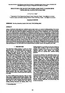
Figure 1. 1. Flowchart Flowchart of of building building point point extraction extraction from from VLS VLS point point data. data. Figure

2. Methods 2. Methods 2.1. Voxel Voxel Group-Based Group-Based Shape Shape Recognition Recognition 2.1. 2.1.1. 2.1.1. Voxelization Voxelization The byby a standard cubecube that that records the serial number of the contained LiDAR The voxel voxelisisrepresented represented a standard records the serial number of the contained points. simple efficient way to way segment point clouds, voxelization has been used inused the LiDAR A points. A but simple but efficient to segment point clouds, voxelization haswidely been widely field forest science. For example, some scholars have segmented thethe ALS ororTLS in theoffield of forest science. For example, some scholars have segmented ALS TLSdata datawith withvoxels voxels to to analyze analyze forest forest structure structure [42,43] [42,43] or or to todescribe describe the themorphological morphological structures structures of tree canopies canopies [44], determine determine crown-base height [45], and separate point clouds into individual trees [46]. Wu et al. [3] [3] used used aa voxel-based voxel-based method method to to extract extract street-lining street-lining trees trees from from VLS VLS LiDAR LiDAR data. data. Wang et al. [47] [47] generated generated DEM DEM using using aa voxel-based voxel-based method. method. Jwa et al. [48] automatically extracted power lines with aa method based based on onvoxelization. voxelization.Owing Owing simplicity ease of representation visually toto itsits simplicity andand ease of representation bothboth visually and and in data structures [49], voxel-based methods havesuitable been suitable for model reconstruction by in data structures [49], voxel-based methods have been for model reconstruction by LiDAR LiDAR data. et al. [50], Hosoi et Stoker al. [51], and Stokervoxel-based [52] adopted voxel-based to data. Park et al.Park [50], Hosoi et al. [51], and [52] adopted methods to buildmethods 3D models build 3D models individual trees, Chengmethods using voxel-based methods for reconstruction of large of individual trees,ofCheng using voxel-based for reconstruction of large multilayer interchange multilayer urban power [54] while some scholars have applied it for bridge [53]interchange and urbanbridge power[53] lineand [54] while someline scholars have applied it for building-model building-model reconstruction with several good results [44–47]. reconstruction with several good results [44–47]. 2.1.2. 2.1.2. Generating Generating of of Voxel Voxel Group Group Voxel-based Voxel-based methods methods can can transform transform the the extraction extraction of of disorderly disorderly distributions distributions of of discrete discrete points points into the filtering of voxels with topological relations [54]. This approach is suitable for vehicle LiDAR into the filtering of voxels with topological relations [54]. This approach is suitable for vehicle LiDAR points. dealing with large-scale urban LiDAR data, the large of voxelsofremains points. However, However,when when dealing with large-scale urban LiDAR data, thevolume large volume voxels an obstacle for rapid process. Therefore a new structure called the “voxel group” has been put forward remains an obstacle for rapid process. Therefore a new structure called the “voxel group” has been to further organize voxels; each voxel group is voxel composed of is several voxelsofthat are adjacent to each put forward to further organize voxels; each group composed several voxels that are other andto have theother sameand geometric properties, as shown in Figure 2. group construction is group based adjacent each have the same geometric properties, asVoxel shown in Figure 2. Voxel on the following two assumptions: (1) A series of voxels with(1) theAsame horizontal coordinates, with construction is based on the following two assumptions: series of voxels with the same elevations adjacent to each other, have a greater possibility of belonging to the same single real-world horizontal coordinates, with elevations adjacent to each other, have a greater possibility of belonging object, as depicted Figure 2b;object, (2) One and in theFigure adjacent with small differences to the same single in real-world asvoxel depicted 2b;voxels (2) One voxel andelevation the adjacent voxels are more likely belong to the same object, as shown in Figure 3d. The above two hypotheses are derived with small elevation differences are more likely belong to the same object, as shown in Figure 3d. The

above two hypotheses are derived from the respective facts that the object’s structure has continuity in vertical directions, regardless whether it is an artificial or natural object.


4 of 25

from the respective facts that the object’s structure has continuity in vertical directions, regardless whether it is an artificial or natural object.


Figure Figure2. 2. Construction Construction of of voxel voxel group. group. (a) (a) Point Point clouds clouds distribution distributionof of several severalobjects objectsin inaa3D 3D voxel voxel grid gridsystem; system;(b) (b)Street Streetlamp lamppoint pointclouds cloudsand andthe thegenerated generatedvoxels; voxels;This Thisisisaatypical typicalcase casein inwhich whichthe the voxels voxelswith withthe thesame samehorizontal horizontaland andvertical verticalcoordinates coordinateswith withadjacent adjacentelevations elevationsbelong belongto tothe thesame same target; target;(c) (c)Schematic Schematicof ofthe theprocess processof ofdividing dividingthe thevoxel voxeldistributions distributionson onthe thesame samevertical verticaldirection; direction; (d)Profile Profileof ofpart partcanopy canopyof ofaastreet streettree, tree, aacase casethat thatadjacent adjacentvoxel voxelwithin withinpoints pointsbelong belongto toone oneobject object (d) havelittle littleelevation elevationdifferences. differences. have

The Theprocess process of of establishing establishing aa voxel voxel group group is is as as below. below. Step Step1: 1:Building Building3D 3Dvoxel voxelgrid gridsystem. system.Set Setan anappropriate appropriatesize sizeSSto tobuild buildaaregular regular3-D 3-Dvoxel voxelgrid grid system. Each LiDAR point is added to each voxel according to its 3D coordinates. The minimum system. Each LiDAR point is added to each voxel according to its 3D coordinates. The minimum value value among all LiDAR coordinates ) is the origin of the 3D voxel grid system. m inthe origin of the 3D voxel grid system. For among all LiDAR pointpoint coordinates px ,( yx m in ,, yzm in ,qz is min

min

min

of its corresponding are For LiDAR point, the row, column, and number layer number (i , its j , k )corresponding eacheach LiDAR point, the row, column, and layer pi, j, kq of voxel arevoxel recorded to construct a two-way index. index. recorded to construct a two-way Step 2: Dividing voxels ineach each column column (in (in vertical vertical direction). direction). On On account account of of aa series series of of voxels voxels Step 2: Dividing voxels in distributed in the same vertical the same row and column pi, jq( imay distributed vertical direction, direction,the thegroup groupofofvoxels voxelswith with the same row and column , j) belong to a different target, such as pedestrians or vehicles below the canopy of trees along a street. may belong to a different target, such as pedestrians or vehicles below the canopy of trees along a Therefore, these voxels must be separated to ensure that each voxel only one object’s street. Therefore, these voxels must be separated to ensure that eachgroup voxel contains group contains only one points, as shown in Figure 2c. Accordingly, the elevation difference between voxel Vpi,j,kq and the voxel object’s points, as shown in Figure 2c. Accordingly, the elevation difference between voxel V( i , j ,k) above it, Vpi,j,k`1q should be calculated: and the voxel above it, V( i , j ,k +1) should be calculated: Dpk,k`1q “ EOPk`1 ´ EOPk (1)

D(k,k+1) = EOPk+1 − EOPk

(1)

EOPk +1 indicates the maximum value of the LiDAR point elevation contained within voxel

V(i , j ,k +1) , and

E O Pk

represents the maximum value of the LiDAR point elevation contained within


5 of 25

EOPk`1 indicates the maximum value of the LiDAR point elevation contained within voxel Vpi,j,k`1q , and EOPk represents the maximum value of the LiDAR point elevation contained within voxel Vpi,j,kq . Threshold Ts is to be set and if Dpk,k`1q ď TS , then Vpi,j,k`1q will join the voxel column, including ! ) ! ) Vpi,j,kq , S “ . . . vpi,j,nq , . . . vpi,j,kq , to form a new voxel column, S “ . . . vpi,j,nq , . . . vpi,j,kq , vpi,j,k`1q . Step 3: Merging process in horizontal direction for voxel group. A full λ-Schedule algorithm is to be taken to merge the voxel columns in horizontal direction. The full λ-Schedule algorithm [55] was first used to segment SAR images. The segmentation principle is based on the Mumford–Shah energy equation to judge the difference in object attributes and the complexity of the object boundary [11]. The merging cost value ti,j of each adjacent voxel column pSi , S j q is calculated as below: ˇ

ˇ

|SiA |¨ˇˇS jA ˇˇ

ti,j

ˇ ˇ ||S E ´ S E || i j |SiA |`ˇˇS jA ˇˇ ` ` ˘˘ “ ` B Si , S j

(2)

pSi , S j q are two adjacent voxel columns in horizontal direction. SiA is the horizontal projection area of voxel column, which is calculated by the defined length l, width w and the number of the horizontal projection grids. SiE is the elevation value of the highest LiDAR point within voxel column. ` ` ˘˘ ` B Si , S j is the length of the shared boundary consists of two parts: the length in vertical direction and the length in horizontal direction. The details are as below: i ii iii iv v

Take a simple region growth for whole voxel columns in horizontal direction based on connectivity to get several rough clusters: tC1 , C2 , . . . , Cn , . . .u. Compute all the pairs of adjacent voxel columns within Cn and their merging cost value from Equation (6) and sort them into a list. Merge the pair (Si ,Sj ) which own smallest ti,j to form a new voxel column Sij and update the merging cost value. Repeat the step ii and step iii until the ti,j exceeds the threshold TEnd or all the voxel columns within Cn into one group. Repeat the step ii, iii, iv until all clusters are processed.

The proposed method take a connectivity-based region growth as first in Step 3 is because the computational complexity of the full λ-Schedule algorithm is o(mglog2 (mn))for a 2D image of m ˆ n pixels [56]. For 3D voxel grid system, the computational complexity will be higher so the origin 3D voxel grid system must be divided into pieces to reduce the amount of involved voxel columns in one process. Finally, all voxel columns are combined into a higher-level structure, the voxel group. The LiDAR points within each voxel group belong to the same single real-world object and have the same geometric properties or shape information.

Remote Sens. 2016, 8, 419 Remote Sens. 2016, 8, 419

6 of 25

Figure of of voxel groups. Figure3.3.Flowchart Flowchartofofgenerating generating voxel groups.


7 of 25

2.1.3. Shape Recognition of Each Voxel Group Demantke et al. [35] and Yang et al. [36] used a PCA-based method to identify the shapes of point clouds. They divided whole point clouds into three categories—linear, planar, and spherical and proved that fusion of point clouds shape information can efficiently segment mobile laser-scanning of point clouds of large-scale urban scenes into single objects. PCA is a common method for analyzing the spatial distributions of neighborhoods of points. It results in a set of positive eigenvalues: λ1 , λ2 , λ3 , pλ1 ą λ2 ą λ3 q. Then Demantke et al. [35] proposed the dimensionality features to describe linear (a1d ), planar (a2d ) and spherical ((a3d )) within. Vp R . Vp R represents the neighboring points of point p with the neighborhood size R. ? ? λ1 ´ λ2 ? a1d “ (3) λ1 ?

a2d “

?

λ? 2 ´ λ3 λ1

?

a3d “ ?λλ3

(4)

(5)

1

A proper neighborhood size is the key for good shape recognition results. Demantke et al. [35] proposed an entropy function that equations the dimensionality of features derived from the eigenvalues of each point: E f pVp R q “ ´a1d lnpa1d q ´ a2d lnpa2d q ´ a3d lnpa3d q

(6)

When E f pVp R q achieve the minimum value, Vp R have the most possibility belong to one dimensionality feature: dpVp R q “ argmaxpand q (7) nPr1,3s

To acquire the optimal neighborhood size of each point, an initial neighborhood size value must be set; it is then gradually increased until the entropy function attains the minimum value. Yang et al. [36] fused the intensity of each point in the process of determining the best neighborhood size to improve the accuracy of estimation of shape features. Both two methods required several calculations of eigenvectors and eigenvalues for each point when the neighborhood size changes; therefore, it is time-consuming and not suitable for handling large-scale urban LiDAR data, even though it can achieve a high accuracy. Unlike the work of Demantke et al. [35] and Yang et al. [36], this article proposes a simple and rapid approach that takes advantage of the voxel group concept for estimation of shape features. The flowchart is shown in Figure 4. Each voxel group is taken as a unit to be estimated its shape. To speed up the process of shape estimation, a part of points in a voxel group is selected instead of its whole points. Because each voxel group may contain point clouds of one tiny single real-world object or a local part of one large single real-world object, the points within one voxel group should have same geometric properties or shape features. The detailed procedure for shape features identifying can be described as follows.

Ropt = arg min( E f (Vp R ))

(9)

R∈ Rmin , Rmax 

Then the dimensionality feature of Vp

Ropt

can be identified by Equation (7). The voxel group and


8 of 25

the whole points within it will be labeled the same dimensionality feature.

Step 1

Voxel Group

Step 2 Determine the range of

Calculate the center

Find the center voxel

neighborhood size [ Rmin , Rmax ]

coordinate

Calculate the

Calculate the

PCA with the points in

entropy feature

dimensionality features

neighborhood R

R < Rmax

Set R =Rmin

R =R +Ri

Yes

No Determine the optimal

Optimal

Labeling all the points in

neighborhood size

dimensionality feature

this voxel group

Step 3

Figure 4. 4. Flowchart Flowchart of of shape shape recognition recognition for for each each voxel voxel group. group. Figure

Every group point clouds are divided into three shapeone categories: linear, Step 1:voxel Finding the and center voxel. Thewithin point it density of each voxel within voxel group is planar and spherical (see Figure 5d) by the Step 1–3 above. The principal direction of point clouds in calculated and finds the most dense voxel Vmd . Calculate the center coordinate of points in this voxel: n ř

`

˘

X, Y, Z “ p

i“0

n

n ř

xi ,

i “0

n

n ř

yi ,

i“0

n

zi q

(8)

` ˘ Step 2: Determine the variation range of neighborhood size. Centering on X, Y, Z , the minimum neighborhood size Rmin is determined as the radius that includes the minimal number Np of points required for PCA. Set the increment Ri , the neighborhood size will increase until the radius reach the boundary of voxel group. Then the variation range of neighborhood size rRmin , Rmax s is obtained. Step 3: Calculate the dimensionality features and entropy feature. Then the dimensionality features a1d , a2d , a3d and entropy feature E f pVp r q within VpR (R P rRmin , Rmax s) are calculated by the Equation (9). In this paper, P denotes the center coordinate of points in the selected voxel. Then the optimal neighborhood size can be obtained: Ropt “ argminpE f pVp R qq

(9)

RPr Rmin ,Rmax s

Then the dimensionality feature of Vp Ropt can be identified by Equation (7). The voxel group and the whole points within it will be labeled the same dimensionality feature. Every voxel group and point clouds within it are divided into three shape categories: linear, planar and spherical (see Figure 5d) by the Step 1–3 above. The principal direction of point clouds


9 of 25


in a linear voxel group, the surface normal direction of point clouds a planar voxel group, and a linear voxel group, the surface normal direction of point clouds in ainplanar voxel group, and thethe coordinates of center point clouds in a spherical voxel group can be further obtained. coordinates of center point clouds in a spherical voxel group can be further obtained.

(a)

(b)

Linear Surface Spherical

(c)

(d)

Figure 5. Voxel group-based shape recognition. (a)(a) Raw LiDAR point clouds include building facades, Figure 5. Voxel group-based shape recognition. Raw LiDAR point clouds include building facades, street trees, street lamps, cars, and the ground; (b) Generated voxel group, voxels of the same color street trees, street lamps, cars, and the ground; (b) Generated voxel group, voxels of the same color belong to the same voxel group; (c) LiDAR points within each voxel group, points of the same color belong to the same voxel group; (c) LiDAR points within each voxel group, points of the same color belong to to thethe same voxel group; (d)(d) Shape recognition results. belong same voxel group; Shape recognition results.

2.2. Category-Oriented Merging 2.2. Category-Oriented Merging AsAs noted, each voxel group and thethe point clouds within it are divided into one shape category: noted, each voxel group and point clouds within it are divided into one shape category: linear, planar, or spherical. The proposed method merges discrete voxel groups into a single reallinear, planar, or spherical. The proposed method merges discrete voxel groups into a single real-world world onground the ground the shape information for building detection. This process objectobject on the fusionfusion of the of shape information for building detection. This process includes includes two steps: removing ground points and category-oriented merging. two steps: removing ground points and category-oriented merging. 2.2.1. Removing Ground Points 2.2.1. Removing Ground Points When addressing outdoor 3D3D data, anan estimate ofof the When addressing outdoor data, estimate theground groundplane planeprovides providesananimportant important contextual cue [57]. in in large-scale urban regions, advance ground point removal can contextual cue [57].Particularly Particularly large-scale urban regions, advance ground point removal can greatly reduce the amount ofof data and improve efficiency. AA simple strategy is is used toto quickly filter greatly reduce the amount data and improve efficiency. simple strategy used quickly filter ground points based onon the establishment ofof the voxel group and shape recognition. The steps ofof this ground points based the establishment the voxel group and shape recognition. The steps this strategy are outlined below. strategy are outlined below. Extracting thethe potential voxel group that contains . The difference value Step 1: 1: Step Extracting potential voxel group that containsground groundpoints points. The difference value between the lowest and highest points is calculated for each planar voxel group with an angle between the lowest and highest points is calculated for each planar voxel group with an angle between ˝: between the surface vector and horizontal plane that is greater 85°: the surface normalnormal vector and horizontal plane that is greater than 85than

D = P hmax− P Dmax ´hmin Phmin max “ hPmax

(10)(10)

Ph min is the elevation value of the lowest point. is the elevation value of the highest point andand is the elevation value of the highest point Phmin is the elevation value of the lowest point. Step 2: Combining the connected region. If the elevation difference between two adjacent candidate voxel groups contains ground points less than 0.3 m, then the two voxel groups are merged. Repeat this process and calculate the area of the final combined voxel group: Ph P max

hmax


10 of 25

Step 2: Combining the connected region. If the elevation difference between two adjacent candidate voxel groups contains ground points less than 0.3 m, then the two voxel groups are merged. Repeat this process and calculate the area of the final combined voxel group: Area “ N ˆ S2

(11)

where N is the number of voxels within the combined voxel group. Step 3: Removing ground points. Set the area threshold 10 m2 to filter the too small combined voxel group. Then all candidate voxel groups’ average elevation are recorded and the outliers are rejected, always indicating the suspended flat roof. All the points within the rest of candidate voxel groups will be labeled as ground points and need to be removed before the next step. 2.2.2. Category-Oriented Merging A single real-world object may consist of more than one shape, such as a building composed of a planar roof and linear columns. Therefore, different rules are set for merging adjacent voxel groups containing non-ground points that have the same or different shape properties based on a region growing algorithm. There come several combinations according to the type of the candidate voxel group: (1) two linear voxel group; (2) two planar voxel group; (3) two spherical voxel group; (4) one linear and one planar voxel group; (5) one linear and one spherical voxel group. Generally, components of artificial objects are approximate parallel or perpendicular to each other, such as palisade tissue, billboard and its stanchion, traffic sign’s cross arm and upright, building’s flashing and facade. When dealing with the combination 1, 2, 4, the principal direction differences or normal vector differences between the two linear voxel groups or two planar voxel groups and the angle differences between the principal direction of the linear voxel group and the normal vector of the planar voxel group firstly. Two parallel candidate voxel groups (differences smaller than 10˝ ) will be required corresponding judging conditions different from the two candidate voxel groups perpendicular to each other. The merging rules are shown in Table 1. Table 1. Rule of merging adjacent voxel groups. Linear Ñ Ñ ps , pˇ c

Linear

If: arccosθ ąď 10˝ ˇ ă && ˇets ´ et p ˇ ď Te && ||os px, y, zq ´ o p px, y, zq|| ă To Ñ Ñ

Else if: arccosθ ă ps , pc ąě 80˝ && S Min ď Tmd Ñ Ñ

Planar

If: arccosθ ă ns , pc ąď 10˝ Ñ Ñ || arccosθ ă ns , pc ąě 80˝ && S Min ď Tmd

Spherical

If: ||os px, yq ´ o p px, yq|| ă To

Ñ Ñ ps , ns ,

Planar

Spherical

Ñ Ñ

If: arccosθ ă ps , nc ąď 10˝ Ñ Ñ || arccosθ ă ps , nc ąě 80˝ && S Min ď Tmd

If: ||os px, yq ´ o p px, yq|| ă To && S Min ď Tmd

Ñ Ñ

˝ If: arccosθ ˇ ă ns , nˇ c ąď 10 && ˇets ´ et p ˇ ď Te Ñ Ñ

Else if: arccosθ ă ns , nc ąě 80˝ && S Min ď Tmd If: ||os px, y, zq ´ o p px, y, zq|| ă To

ets and os px, y, zq respectively denote the principal direction, surface normal, top elevation, center coordinates, and the radius of the seed voxel group. The bottom-left voxel group is usually Ñ Ñ selected as the seed voxel group. The pc , nc , etc , oc px, y, zq denote the principal direction, surface normal, the top elevation and the center coordinates of the candidate voxel group in seed voxel group’s neighborhood. S Min represents the minimum euclidean distance between the seed voxel group and candidate voxel group, which indicate whether two candidate voxel group are connect. Te , To and Tmd are the corresponding threshold values of each condition. The merging result of testing area without ground points as shown in Figure 6. As can be seen from Figure 6, voxel groups of one single real-world object with same or different shape can merge


The merging result of testing area without ground points as shown in Figure 6. As can be seen of 25 groups of one single real-world object with same or different shape can11merge together. For example, Figure 6b shows that the parallel linear voxel groups, linear voxel groups perpendicular to each other and the planar voxel groups representing of one bus stop’s components together. For example, Figure 6b shows that the parallel linear voxel groups, linear voxel groups can merge well. Figure 5d shows that two planar voxel groups perpendicular to each other perpendicular to each other and the planar voxel groups representing of one bus stop’s components can representing of one building’s corner can merge together. Figure 6e shows that one linear voxel group merge well. Figure 5d shows that two planar voxel groups perpendicular to each other representing of representing of one tree’s trunk and several spherical voxel groups representing of tree’s canopy can one building’s corner can merge together. Figure 6e shows that one linear voxel group representing of merge well also. one tree’s trunk and several spherical voxel groups representing of tree’s canopy can merge well also. Remote 2016,6,8, voxel 419 fromSens. Figure

Figure6.6.Category-oriented Category-orientedmerging. merging.(a) (a)Merging Mergingresults, results,points pointsofofthe thesame samecolor colorbelong belongtotothe thesame same Figure segment;(b–e) (b) (c) (d) (e)real-world I: Single real-world object with several voxel groups, points the same color segment; I: Single object with several voxel groups, points of the sameofcolor belong to belong the group; same voxel group; II: Shapes object, red points, denotesgreen lineardenotes points,surface green denotes the same to voxel II: Shapes of one object, of redone denotes linear points, and blue points, denotesand spherical points. spherical points. surface blue denotes

2.3.Horizontal HorizontalHollow HollowRatio-Based Ratio-BasedBuilding BuildingPoint PointIdentification Identification 2.3. Thelaser laserscanner scannercan cangive giverich richsurface surfaceinformation informationofofobjects objectsbut butcouldn’t couldn’tpenetrate penetratethe thesurface. surface. The Due to that fact, Aljumaily et al. [58] found out that each building appears as a deep hole by viewing Due to that fact, Aljumaily et al. [58] found out that each building appears as a deep hole by viewing thebottom bottomview viewofofthe theDEM DEMgenerated generatedby byALS ALSdata. data.InInaddition, addition,he heextracted extractedbuilding buildingusing usingthis this the character. It is indicated that the defects of LiDAR data can be transformed into some advantages that character. It is indicated that the defects of LiDAR data can be transformed into some advantages cancan be utilized. VLSVLS building point clouds primarily remain on on thethe facade butbut areare lacking in the top that be utilized. building point clouds primarily remain facade lacking in the andand inner structures because of building buildingmaterials. materials. top inner structures becauseofofscanner scannerangle angleconstraints constraintsand and the the resistance resistance of Compared to objects commonly found in urban environments, such as vehicles or street trees, the Compared to objects commonly found in urban environments, such as vehicles or street trees, the ratio ratio the building pointprojection cloud projection area occupies, which is surrounded by theis contour, that thethat building point cloud area occupies, which is surrounded by the contour, relativelyis relatively small. In other from top view, building clouds are more “hollow” thanpoint other small. In other words, fromwords, top view, building point cloudspoint are more “hollow” than other object object point clouds, as shown in Figure 7. clouds, as shown in Figure 7. As shown in Figure 7, a patch with a different color represents the range of particular a convex hull generated by each segment’s point clouds. It can be directly found out that the area occupied by building’s point clouds is much smaller than the area of convex hull while tree and car have the


opposite situation. Remote Sens. 2016, 8, 419 For a more accurate analysis, the horizontal hollow ratio of every object12is of 25 presented in Figure 8 to compose a graph as follows.

(a)

(b)

(c) Figure Horizontalhollow hollowratio-based ratio-basedbuilding building point top view of segments Figure 7.7. Horizontal point identification identification(a–c). (a–c).Left: Left: top view of segments of point clouds of several buildings, trees and cars. Right: overlay of a convex hull and point clouds of point clouds of several buildings, trees and cars. Right: overlay of a convex hull and point clouds of of each segment. each segment.

As shown in Figure 7, a patch with a different color represents the range of particular a convex hull generated by each segment’s point clouds. It can be directly found out that the area occupied by building’s point clouds is much smaller than the area of convex hull while tree and car have the opposite situation. For a more accurate analysis, the horizontal hollow ratio of every object is presented in Figure 8 to compose a graph as follows.


13 of 25

Figure Figure 8. 8. Horizontal Horizontal hollow hollow ratios ratios of of buildings, buildings, cars, cars, and and trees trees in in Figure Figure 66 (one (one point point represents represents one one object object in in Figure Figure 6). 6).

X-axis (NACH Ratio) represents the normalization ratio between the area of each object’s convex X-axis (NACH Ratio) represents the normalization ratio between the area of each object’s convex hull and the maximum convex hull area common to this type of object. This ratio indicates hull and the maximum convex hull area common to this type of object. This ratio indicates the the morphological changes of objects. The Y-axis represents the horizontal hollow ratio. The morphological changes of objects. The Y-axis represents the horizontal hollow ratio. The horizontal horizontal hollow ratio of tree is very close to the horizontal hollow ratio of car while building’s hollow ratio of tree is very close to the horizontal hollow ratio of car while building’s horizontal hollow horizontal hollow ratio is significantly smaller than that of the other two kinds. A detailed procedure ratio is significantly smaller than that of the other two kinds. A detailed procedure for building points for building points extraction based on horizontal hollow ratio can be described as follows. extraction based on horizontal hollow ratio can be described as follows. Step 1: Extracting outline. The proposed method makes every segment’s voxels project to the Step 1: Extracting outline. The proposed method makes every segment’s voxels project to the horizontal plane to form two-dimensionality grids and employ the simple and efficient method horizontal plane to form two-dimensionality grids and employ the simple and efficient method proposed by Yang [1] to extract the contour grid: if eight neighbor grids of one background grid proposed by Yang [1] to extract the contour grid: if eight neighbor grids of one background grid (contains no points) are not all background grid, it will be labeled as contour grid. The aim of this (contains no points) are not all background grid, it will be labeled as contour grid. The aim of this step step is to reduce the amount of calculation in next step. is to reduce the amount of calculation in next step. Step 2: Generating convex hull. When get the contour grids of one segment, the convex hull of Step 2: Generating convex hull. When get the contour grids of one segment, the convex hull of this segment is calculated by the Graham’s Scan method. Furthermore, the convex hull area S C of this segment is calculated by the Graham’s Scan method. Furthermore, the convex hull area SC of this this segment cancalculated. be calculated. segment can be Step 3: Calculating . The Step 3: Calculatinghorizontal horizontalhollow hollowratio ratio. Theproposed proposedmethod methoddefines definesthe thehorizontal horizontal hollow hollow ratio ratio of of each each voxel voxel cluster cluster to to indicate indicate the the above above feature: feature: SSgg RRHH“= S SCC

(12) (12)

Sg isisthe thearea areaofofthis thissegment’s segment’stwo-dimensionality two-dimensionalitygrids: grids: S g S = N × l× w

g Sg “ Nˆlˆw

(13) (13)

where N is the number of two-dimensionality grids. where N is4:the number of threshold two-dimensionality Step Calculating . OTSU is grids. an automatic and unsupervised threshold selection Step 4: Calculating threshold. is an automatic and unsupervised threshold method. Based on this method, theOTSU optimal threshold selection should be made with selection the best method. Based on this method, the optimal threshold selection should be made with the best separation separation of the two types obtained by the threshold segmentation. The interclass separability of the twoistypes by the threshold The interclass separability criterion is the best criterion the obtained best statistical differencesegmentation. between class characteristics of maximum or minimum statistical difference between class characteristics of maximum or minimum differences within class differences within class characteristics [59]. The building’s hollow ratio is far smaller than that of characteristics [59]. The building’s hollow ratio is far smaller than that of other objects, as indicated by other objects, as indicated by Figure 7; therefore, using the OTSU method to obtain threshold T of the Figure 7; therefore, using the OTSU method toobjects obtain should threshold T of the hollow ratio of the divided hollow ratio of the divided building and other achieve a good effect: building and other objects should achieve a good effect: T = Arg Max”  PA (ωA − ω0 )2 + PB (ωB − ω0 )2  ı (14) 0 ≤ t ≤ L −1 T “ Arg Max PA pω A ´ ω0 q2 ` PB pω B ´ ω0 q2 (14) 0 ď t ď L ´1 where L is the maximum value of the hollow ratio among all the voxel clusters, and PA and P B are the probabilities of respective building voxel clusters and non-building voxel clusters. ω A and


14 of 25

where L is the maximum value of the hollow ratio among all the voxel clusters, and PA and PB are the probabilities of respective building voxel clusters and non-building voxel clusters. ω A and ω B are the average hollow ratio values of building voxel clusters and non-building voxel clusters. Only voxel clusters with the average height of H ě 2.5m and cross-sectional area of Csa ą 3m2 are used by the OTSU algorithm. If a voxel cluster’s hollow ratio is less than threshold T, it is deemed a building voxel cluster and all points within it are considered building points. 3. Results and Discussion The algorithm proposed was programmed in C# on Microsoft Visual Studio platform. The hardware system was a computer with 8 GB of RAM and a quad-core 2.40 GHz processor. 3.1. Study Area and Experimental Data The region of the Olympic Sports Center, Jianye District, Nanjing City, China, is chosen as the experimental area (Figure 9). To capture the vehicle LiDAR data, we employed an SSW mobile mapping system, developed by Chinese Academy of Surveying and Mapping, with a 360˝ scanning scope, a surveying range of 3 to 300 m, reflectance of 80%, and a point frequency of 200,000 points/s. The survey was conducted in 2011 and a topographic map of 1:500 was used for data correction. The overall data were approximately 4 GB, which covered a 1.4 km ˆ 0.8 km area with 147,478,200 points. The point density is 270 points/m2 . Due to the amount of testing data being huge, the proposed method is unable to process it in one time. Therefore, we clip the raw testing data into 12 parts according to the road segments in practice. The experimental region contained both downtown area and urban residential area with a number of commercial and residential architecture. A shopping mall, a skyscraper, an apartment building, and a high-rise office building are the main architecture buildings in the study area. Due to the good road greening, a large number of street trees exist in the study area, which cause strong variation of point densities of building façade. On the other hand, it is sometimes difficult separate the buildings and the trees surround it.

Figure 9. Experimental area. (a) Aerial orthophotos of the experimental area, red line denotes the SSW mobile mapping system’s driving route; (b) Raw VLS data of the experimental area.


15 of 25

The proposed method consists of four parts: Voxel group generating, shape recognition, category-oriented merging, and building points identification. As a few parameters and thresholds are set in each part, the summarization on the setting of the key parameters and threshold is given in Table 2. The setting basis of these thresholds and parameters includes three types: data source, calculation, and empirical. The term “data source” indicates that the values are adjusted according to the experimental data and area. The term “calculation” means that the values are calculated automatically. As for the term “empirical”, it means that the values are set empirically. In the proposed method, they are always controlled by the voxel size. The value set according to data source can be determined based on the shape property and the distribution of the objects in the experimental area. However, the optimal value set according to empirical must to be determined by several repeated test. This is the main difference among “data source” and “empirical”. Table 2. The key thresholds and parameters of the proposed approach.

Voxel group generating

Shape recognition

Category-oriented merging

Building point identification

Items

Values

Description The voxel size To divide the adjacent voxel in vertical direction To terminate the growth of voxel groups’ generating

S

0.5 m

TS

0.2 m

TEnd

0.85

Np Ri

5 pts 0.1 m

Te

0.1 m

To

0.5 m

Tmd

0.15 m

T

Automatic

H

2.5 m

Csa

3

m2

Minimum number of points for PCA The increment of the search radius Maximal difference of elevation between two voxel groups Maximal distance between two voxel groups’ center Maximal minimum euclidean distance between two voxel groups The threshold of the horizontal hollow ratio to identify building points Minimum average height of voxel cluster Minimum Cross-sectional area of voxel cluster

Setting Basis Empirical Data source Chen et al. [11] Empirical Empirical Data source Empirical Data source Calculation Data source Data source

During the generating of voxel group, we set the size S = 0.5 m to form a regular 3-D voxel grid. The size of the voxel is closely related to the extraction of the building points. Some of the buildings lost part of the facade and other appendants, like the podium building, when the voxel size is too small. If the voxel size chosen is too large, the tree and brush close to the building will be classified to building points incorrectly. Some small and low-rise building will be identified as tree or brush due to the same reason. On the other hand, the smaller the voxel size is, the long the execution time is. The threshold to divide the adjacent voxel in vertical direction is set according to the data source. The threshold to terminate the growth of voxel groups’ generating is set according to Chen et al. [11]. By this test, 0.85 is the best value. During the shape recognition of the points in each voxel group, the minimal number of points to initialize the minimum search radius and the increment of the search radius is set empirically. The voxel size is one influential factor of the values. During the category-oriented merging with voxel groups, voxel groups are merged by utilizing the shape information on several rules. The maximal difference in elevation, maximal minimum Euclidean distance between two voxel groups can be setting according to the data source. The maximal distance between two voxel groups’ centers can be set empirically. This value is depending on the voxel size. The bigger the voxel size was set, the greater the value.


maximal distance two voxel groups’ centers can be set empirically. This value is depending Remote Sens. 2016, 8, between 419 16 of 25 on the voxel size. The bigger the voxel size was set, the greater the value. During the building point identification, the horizontal hollow ratio of each voxel cluster meets During the building point identification, the horizontal hollow ratio of each voxel cluster meets the conditions is calculated. The threshold of the horizontal hollow ratio to identify building points the conditions is calculated. The threshold of the horizontal hollow ratio to identify building points is calculated automatically by the OTSU method. The minimum average height and the minimum is calculated automatically by the OTSU method. The minimum average height and the minimum cross-sectional area of voxel clusters need to be set according to the data source. These two values are cross-sectional area of voxel clusters need to be set according to the data source. These two values are the approximate size of a newsstand, which can be often viewed along the urban street of Nanjing the approximate size of a newsstand, which can be often viewed along the urban street of Nanjing and and be considered as the smallest building. be considered as the smallest building. 3.2. Extraction Results of Building Points 3.2. Extraction Results of Building Points The raw vehicle LiDAR point clouds and aerial orthophotos are used to manually extract the The raw vehicle LiDAR point clouds and aerial orthophotos are used to manually extract the building points. The aerial orthophotos were acquired at the same time period when collecting building points. The aerial orthophotos were acquired at the same time period when collecting LiDAR LiDAR data and they can be matched. The spatial resolution of the aerial orthophotos is 0.2 m and data and they can be matched. The spatial resolution of the aerial orthophotos is 0.2 m and presented presented in 3 bands red-green-blue (RGB). The extraction results were then used as the validation in 3 bands red-green-blue (RGB). The extraction results were then used as the validation data. Building data. Building point boundaries were connected to determine the building regions as the ground point boundaries were connected to determine the building regions as the ground truth, referred truth, referred to herein as the true building region. Figure 10 illustrates the extraction results of to herein as the true building region. Figure 10 illustrates the extraction results of building points. building points. LiDAR points are marked in blue for buildings, red for the ground, and green for LiDAR points are marked in blue for buildings, red for the ground, and green for the other features. the other features. As shown in Figure 10b–d, our method extracted not only high-rise and low-rise As shown in Figure 10b–d, our method extracted not only high-rise and low-rise buildings, but also buildings, but also buildings with special exteriors or complex structures. Moreover, as shown in buildings with special exteriors or complex structures. Moreover, as shown in Figure 10e, the proposed Figure 10e, the proposed method recognized buildings with missing parts of facade that were caused method recognized buildings with missing parts of facade that were caused by field measurement by field measurement conditions or equipment factors. The SSW vehicle-borne laser scanning system conditions or equipment factors. The SSW vehicle-borne laser scanning system accomplished the accomplished the objective of obtaining 192 relatively complete buildings from the experimental area objective of obtaining 192 relatively complete buildings from the experimental area with a total of with a total of 235 buildings. A relatively complete building refers to the scanning point cloud of the 235 buildings. A relatively complete building refers to the scanning point cloud of the building with building with at least two facades. The types of buildings in the study area included low cottages, at least two facades. The types of buildings in the study area included low cottages, middle-rise middle-rise residential buildings, high-rise commercial buildings, and unique structures, such as residential buildings, high-rise commercial buildings, and unique structures, such as bell towers bell towers and theaters. and theaters.

(a)

(c) (b) Figure 10. Cont.


17 of 25

(d)

(e)

Figure10.10.Building Buildingpoint pointextraction extractionresults. results.(a) (a)Extraction Extractionresults resultsofofbuildings buildingsininthe theexperiment experiment Figure region; (b,c) Proposed method successfully detected various building shapes, including skyscrapers region; (b,c) Proposed method successfully detected various building shapes, including skyscrapers andlow low cottages;(d) (d)Proposed Proposedmethod methodeffectively effectivelyseparated separateda abuilding buildingand andthe thetrees treesattached attachedtotoit;it; and cottages; (e) Results show that the method could also recognize buildings with sparse LiDAR points lack (e) Results show that the method could also recognize buildings with sparse LiDAR points oror lack ofof partial structures. partial structures.

3.3. Evaluation of Extraction Accuracy 3.3. Evaluation of Extraction Accuracy In this section, the extraction accuracy of the proposed method is validated from two aspects: In this section, the extraction accuracy of the proposed method is validated from two aspects: building-based evaluation for overall experimental area (a whole building taken as an evaluation building-based evaluation for overall experimental area (a whole building taken as an evaluation unit) unit) and point-based evaluation for individual building (a point taken as an evaluation unit). To and point-based evaluation for individual building (a point taken as an evaluation unit). To analyze analyze the proposed algorithm in details, this article divided the buildings into three types: lowthe proposed algorithm in details, this article divided the buildings into three types: low- (one to (one to two stories), middle- (three to seven stories), and high-rise structures (more than seven stories). two stories), middle- (three to seven stories), and high-rise structures (more than seven stories). The correctness and completeness of the method are used as indexes for the evaluation, as follows: The correctness and completeness of the method are used as indexes for the evaluation, as follows: TP Completeness = TP (15) Completeness “ TP + FN (15) TP ` FN

TP TP Correctness Correctness “= TP TP`+FP FP

(16)

InInthe theevaluation evaluationfor foroverall overallexperimental experimentalarea, area,where whereTP TPisisthe thenumber numberofoftrue truebuildings, buildings,FPFPisis the number of wrong buildings, and FN is the number of mis-detected buildings. The the number of wrong buildings, and FN is the number of mis-detected buildings. Thebuildings buildings derived byby manual operation areare taken as reference data. By overlaying one extracted building and the derived manual operation taken as reference data. By overlaying one extracted building and corresponding reference data, the overlapped area of them is calculated. If the ratio of this overlapped the corresponding reference data, the overlapped area of them is calculated. If the ratio of this area to area ofarea the to extracted is larger than is 70%, thethan extracted building is taken as true one. overlapped area of building the extracted building larger 70%, the extracted building is taken Otherwise, it is considered as a wrong one. If a building is not be detected by the automatic process, as true one. Otherwise, it is considered as a wrong one. If a building is not be detected by the it automatic is considered to be it a mis-detected process, is considered building. to be a mis-detected building. InIn the evaluation for individual building, where TP TP is the number of true points belonging to it, to FPit, the evaluation for individual building, where is the number of true points belonging isFP theisnumber of wrong points belonging to it, andtoFN the FN number of number mis-detected points belonging the number of wrong points belonging it,isand is the of mis-detected points tobelonging it. The extracted building points and true building points are put together. The points of overlapped to it. The extracted building points and true building points are put together. The points region are regarded as true (blue in Figure points existing only in theexisting truth regions of overlapped region are points regarded as points true points (blue11c); points in Figure 11c); points only in are deemed misdetections (yellow points in Figure 11c), and points existing only in the extracted the truth regions are deemed misdetections (yellow points in Figure 11c), and points existing only in regions are considered points (red points in Figure 11c). in Figure 11c). the extracted regions wrong are considered wrong points (red points


18 of 25

(a)

(b)

Missing Points Correct Points Error Points

(c) Figure 11. 11.Point-based Point-based evaluation individual building. (a) Automatic extraction of a Figure evaluation for for individual building. (a) Automatic extraction results ofresults a building; building; Manual results extraction results the same (c) Overlay result witherror, the correct, error, (b) Manual(b) extraction of the sameof building; (c)building; Overlay result with the correct, and missing and missing points denoted in blue, red, and yellow, respectively. points denoted in blue, red, and yellow, respectively.

3.3.1. Building-Based Evaluation for Overall Experimental Area 3.3.1. Building-Based Evaluation for Overall Experimental Area There are 192 buildings involved in the evaluation in this section, including 42 low-rise buildings, There are 192 buildings involved in the evaluation in this section, including 42 low-rise buildings, 126 medium-rise buildings, and 24 high-rise buildings. 126 medium-rise buildings, and 24 high-rise buildings. As the height of the building increased, the completeness of extraction results increased; the As the height of the building increased, the completeness of extraction results increased; the high-rise buildings’ completeness reached 100%, whereas that of the low-rise buildings reached only high-rise buildings’ completeness reached 100%, whereas that of the low-rise buildings reached only 86.3%. This was due to the low-rise buildings’ top and internal structures being more apt to scanning 86.3%. This was due to the low-rise buildings’ top and internal structures being more apt to scanning by the mobile laser scanner; therefore, the low-rise buildings’ hollow ratios calculated by the by the mobile laser scanner; therefore, the low-rise buildings’ hollow ratios calculated by the algorithm algorithm reached lower values than those of the high-rise buildings. Hence, if a very tall building reached lower values than those of the high-rise buildings. Hence, if a very tall building and a low-rise and a low-rise building were in the same region, the low-rise building with a low hollow ratio may building were in the same region, the low-rise building with a low hollow ratio may have been have been incorrectly identified as a vehicle, bush, or other object. The overall completeness and incorrectly identified as a vehicle, bush, or other object. The overall completeness and correctness were correctness were 94.7% and 91%, respectively. As a comparison, one automatic building detection 94.7% and 91%, respectively. As a comparison, one automatic building detection method reported by method reported by Truong-Hong and Laefer [41] conducted in the similarly dense urban area Truong-Hong and Laefer [41] conducted in the similarly dense urban area achieved 95.1% completeness achieved 95.1% completeness and 67.7% correctness from ALS data. and 67.7% correctness from ALS data. Two primary types of incorrect detections occurred. Firstly, because some vehicles were in highTwo primary types of incorrect detections occurred. Firstly, because some vehicles were in speed motion, these vehicles’ point clouds were stretched, or adjacent vehicles’ point clouds may high-speed motion, these vehicles’ point clouds were stretched, or adjacent vehicles’ point clouds may have merged, which caused them to be incorrectly detected as buildings owing to the high hollow have merged, which caused them to be incorrectly detected as buildings owing to the high hollow ratio values they incurred. Secondly, because their shapes can be similar to building facades, high ratio values they incurred. Secondly, because their shapes can be similar to building facades, high fences resulted in high hollow ratios and they were consequently incorrectly detected as buildings. fences resulted in high hollow ratios and they were consequently incorrectly detected as buildings.


19 of 25

3.3.2. Point-Based Evaluation for Individual Building In this evaluation, to further evaluate the effect of the proposed method, complex buildings are entered into a separate category (a new type of buildings), named complex buildings in Table 2. The individual evaluation results in Table 3 show that the middle-rise buildings have better extraction results than the low-rise and high-rise buildings. The average completeness and correctness of the middle-rise buildings are 95% and 95.7%, respectively. The low-rise buildings yield the worst extraction results, with a completeness and correctness of 94.8% and 93.1%, respectively. These latter results are due to the relative complexity of the vicinities of low-rise buildings; the proposed method employs the voxel group to segment the point clouds. This combined some of the buildings’ point clouds and those of adjacent bushes, trees, and other objects into one group, which reduced the accuracy. Table 3. Completeness and correctness of the extracted building points. Number of Points

Correctness (%)

Average Com (%)

Average Corr (%)

TP

FN

FP

Completeness (%)

Low-rise

15,744 54,399 6750 6830 30,752 38,580 20,751 8048 23,606 12,083

500 2233 0 377 3234 0 1705 0 3234 1473

1239 349 598 135 3827 5122 512 1147 336 1639

96.9 96.1 100 94.8 90.5 100 92.4 100 87.7 89.1

92.7 99.4 91.9 98.1 88.9 88.3 97.6 87.5 98.6 88.1

94.8

93.1

Medium-rise

167,478 85,670 194,255 198,123 125,507 237,798 50,687 219,639 45,340 25,536

934 543 1560 846 6835 11,732 10,466 9897 3699 2229

2126 1408 3210 1042 773 10,592 5872 5396 1146 5587

99.4 99.4 99.2 99.6 94.8 95.3 82.9 95.7 92.5 92.0

98.7 98.4 98.4 99.5 99.4 95.7 89.6 97.6 97.5 82.0

95.0

95.7

High-rise

115,343 186,558 253,489 206,176 209,904 320,217 153,428 144,498 54,596 133,353

14,306 6697 14,368 6467 38,477 26,779 26,186 10,957 9874 9248

388 2993 1152 1388 3387 432 0 0 0 652

89.0 96.5 94.6 97.0 84.5 92.3 85.4 93.0 84.7 93.5

99.7 98.4 99.5 99.3 98.4 99.9 100.0 100.0 100.0 99.5

91.0

99.4

Complex

313,922 34,455 26,540 11,945 17,711 608,188 281,385 282,115 19,957 312,765

22,428 1798 739 4250 2415 24,904 26,653 11,010 832 27,144

1716 254 613 0 136 0 342 2341 687 4336

93.3 95.0 97.3 73.8 88.0 96.1 91.3 96.2 96.0 92.0

99.5 99.3 97.7 100.0 99.2 100.0 99.9 99.2 96.7 98.6

91.9

99.0

Type

The high-rise buildings demonstrate the highest correctness and lowest completeness at 99.4% and 91%, respectively. This is due to the limitation of the scanner angle; i.e., the vehicle-borne laser


20 of 25

scanning system was unable to obtain the point clouds of upper stories and facades that did not face the road. This prevented some of the building point clouds being added to the main part of the building in regional growing process. On the other hand, for high-rise buildings, such as commercial and office buildings, the surrounding environments were relatively simple; objects adjacent to these buildings had very distinct elevations and shapes. Therefore, the high-rise building extraction results had the lowest completeness but highest correctness. The complex buildings have an irregular shape and complicated structure, so it is hard to identify all the parts of a complex building. The complex building’s average completeness is 91.9%, on the whole in a satisfactory level. However, from the ten chosen complex building, it is can be found find that the completeness of each building has a large span, from 73.8% to 97.3%, which indicate that the method may face a challenge when dealing with some special building. 3.4. Experiment Discussion Overall, the detection results in Figure 10 and the evaluation outcomes showed that the proposed method can work well in dense urban areas. The voxels generated by the raw point clouds were divided into voxel columns. A full λ-Schedule algorithm, which considers the complexity of the object boundary, was used for the voxel columns merging and an optimal regularization parameter can be drawn. As a contrast, the termination rules of a 3D region growing approach are difficult to determine. Although the 3D region growing method can construct voxel groups more efficient but the results are always over-segmentation. Five combinations based on two voxel groups’ shapes were presented. Each combination has its own merging rule and high-precise segmentation results were achieved by region growing. The method have more potential for acquiring a further improvement by using machine learning (e.g., Support Vector Machine, SVM) and fusing with intensity or color information of point clouds. The proposed method and the method of Yang et al. [37] show some similarity in the strategy of the segmentation of point clouds, so a comparison was undertaken in this section. The method of Yang et al. [37] generates multi-scale supervoxels from VLS data and segments these supervoxels. Then a set rules was defined for merging adjacent segments with semantic knowledge. We divided both the strategy of the segmentation of point clouds of the proposed method and Yang’s method into three steps: the point organization, shape recognition and merging. Region 5 (red rectangle in Figure 10a) with 458,259 points is the test area for the comparison between the proposed method and Yang’s method. Point clouds are assigned to 1400 voxel groups or 7282 supervoxels. It can be found that the objects with simple structure, like building facade, have greatly fewer voxel groups than supervoxels. There are many more small areas of flat facade of the building were classified into linear or spherical structure incorrectly by Yang’s method. This is due to that the voxel group is bigger than supervoxel in size, so the voxel group can contain more complete structure of the single real-world object. The points of the building are divided into one segment by the proposed method while they were separated into several segments by Yang’s method. Through the comparison of the two methods’ result, the proposed method handles the shape recognition and segmentation of building facade better than the method of Yang et al. [37]. Table 4 shows that the proposed method needs less execution time than Yang’s method in each step. Table 4. Time performance of the proposed method and the method of Yang et al. [37].

The proposed method(s) Yang’s method(s)

Point Organization

Shape Recognition

Merging

Total

4.32 7.67

9.91 10.44

9.45 16.96

23.68 35.07

Figure 12 illustrates the comparative experiments result of building extraction by the proposed method and the method of Yang et al. [37]. Region 4 (red rectangle in Figure 9a) is the test area with


21 of 25

5,298,460 points and five buildings. Both methods extract all buildings and no misclassification error Sens. 2016, 8, 419 has Remote occurred. Figure 12a–c shows that the proposed method can extract more details of the building (see black rectangles), like beam and bay window. Figure 12d,e shows that the proposed method (see black rectangles), like beam and bay window. Figure 12d,e shows that the proposed method can can reduce reducethe theerror errorcaused caused noise around building tree,car) andand car)asand as far as byby thethe noise around the the building (e.g.,(e.g., bush,bush, tree, and far as possible to retain the accessory structures of the building at the same time. On the other hand, possible to retain the accessory structures of the building at the same time. On the other hand, Yang’sYang’s method hashas wrongly ofall allthe theextracted extracted buildings as ground the method wronglyidentified identified the the bottom bottom of buildings as ground pointspoints while while the proposed method avoidsthis thismistake. mistake. proposed method avoids Street image

Raw data

Building extraction result The proposed method Yang’s method

(a)

(b)

(c)

(d)

(e)

Figure Comparisonofofbuilding buildingextraction extraction result method andand the the method Figure 12.12. Comparison resultbetween betweenthe theproposed proposed method method of of Yang et al. [37]. (a–e) Left to right: street image, raw VLS data, the result by the proposed method Yang et al. [37]. (a–e) Left to right: street image, raw VLS data, the result by the proposed method and and the result by Yang’s method of the specific building. the result by Yang’s method of the specific building.


22 of 25

4. Conclusions The study proposed an approach for automatic extraction of building points using vehicle-borne laser scanning data. From experimental results, the following points can be drawn. (1) The proposed approach, including voxel group-based shape recognition, category-oriented merging, and horizontal hollow-based building point identification, can be applied in the various types of buildings, in large-scale and complex urban environments. (2) The category-oriented merging with voxel group-based shape recognition is effective in improving the accuracy of segmentation and to develop the new voxel group structure for accelerating processing and simplifying shape recognition. (3) The concept of horizontal hollow ratio for building point cloud identification can accurately extract various forms of buildings, from low cottages and common residential buildings to the towering skyscrapers and remarkable stylish theaters, without requiring complex semantic rules. This point indicated that some characteristics of LiDAR data caused by the constraints of the laser sensor are not obstacles, but some good indicators for particular objects. This is a new concept in the classification of LiDAR data fields. Our future work will focus on fusing VLS data with ALS data and optical images, such as street images, to obtain more complete and accurate building point detection results. Otherwise, the huge data amount of mobile LiDAR data largely reduces the efficiency of information extraction for specific applications. Future work is to develop high-performance computation technology for mobile LiDAR data processing. Acknowledgments: This work is supported by the National Natural Science Foundation of China (Grant No. 41371017, 41001238), the National Key Technology R&D Program of China (Grant No. 2012BAH28B02). The authors thank the anonymous reviewers and members of the editorial team for their comments and contributions. Author Contributions: Yu Wang and Liang Cheng proposed the core idea of voxel group and horizontal hollow analysis based building points extraction method and designed the technical framework of the paper. Yu Wang performed the data analysis, results interpretation, and manuscript writing. Yang Wu assisted with the experimental result analysis. Yanming Chen and Manchun Li assisted with refining the research design and manuscript writing. Conflicts of Interest: The authors declare no conflict of interest.

Abbreviations The following abbreviations are used in this manuscript: MDPI DOAJ TLA LD

Multidisciplinary Digital Publishing Institute Directory of open access journals Three letter acronym linear dichroism

References 1. 2. 3. 4. 5. 6.

Yang, B.; Wei, Z.; Li, Q.; Li, J. Semiautomated building facade footprint extraction from mobile LiDAR point clouds. IEEE Geosci. Remote Sens. Lett. 2013, 10, 766–770. [CrossRef] Hong, S.; Jung, J.; Kim, S.; Cho, H.; Lee, J.; Heo, J. Semi-automated approach to indoor mapping for 3D as-built building information modeling. Comput. Environ. Urban Syst. 2015, 51, 34–46. [CrossRef] Remondino, F. Heritage recording and 3D modeling with photogrammetry and 3D scanning. Remote Sens. 2011, 3, 1104–1138. [CrossRef] Cheng, L.; Wang, Y.; Chen, Y.; Li, M. Using LiDAR for digital documentation of ancient city walls. J. Cult. Herit. 2016, 17, 188–193. [CrossRef] He, M.; Zhu, Q.; Du, Z.; Hu, H.; Ding, Y.; Chen, M. A 3D shape descriptor based on contour clusters for damaged roof detection using airborne LiDAR point clouds. Remote Sens. 2016, 8, 189. [CrossRef] Cheng, L.; Gong, J.; Li, M.; Liu, Y. 3D building model reconstruction from multi-view aerial imagery and LiDAR data. Photogramm. Eng. Remote Sens. 2011, 77, 125–139. [CrossRef]


7.

8. 9. 10. 11.

12. 13. 14. 15. 16. 17. 18. 19.

20. 21.

22.

23.

24.

25. 26. 27. 28.

23 of 25

Wu, B.; Yu, B.; Yue, W.; Shu, S.; Tan, W.; Hu, C.; Huang, Y.; Wu, J.; Liu, H. A voxel-based method for automated identification and morphological parameters estimation of individual street trees from mobile laser scanning data. Remote Sens. 2013, 5, 584–611. [CrossRef] Rutzinger, M.; Rottensteiner, F.; Pfeifer, N. A comparison of evaluation techniques for building extraction from airborne laser scanning. IEEE J. Sel. Topics Appl. Earth Observ. Remote. 2009, 2, 11–20. [CrossRef] Sampath, A.; Shan, J. Segmentation and reconstruction of polyhedral building roofs from aerial LiDAR point clouds. IEEE Trans. Geosci. Remote Sens. 2010, 48, 1554–1567. [CrossRef] Kim, K.; Shan, J. Building roof modeling from airborne laser scanning data based on level set approach. ISPRS J. Photogramm. Remote Sens. 2011, 66, 484–497. [CrossRef] Yanming, C.; Liang, C.; Manchun, L.; Jiechen, W.; Lihua, T.; Kang, Y. Multiscale grid method for detection and reconstruction of building roofs from airborne LiDAR data. IEEE J. Sel. Topics Appl. Earth Observ. Remote Sens. 2014, 7, 4081–4094. Sun, S.; Salvaggio, C. Aerial 3D building detection and modeling from airborne LiDAR point clouds. IEEE J. Sel. Topics Appl. Earth Observ. Remote. 2013, 56, 1440–1449. [CrossRef] Rottensteiner, F. Automatic generation of high-quality building models from LiDAR data. IEEE Comput. Graphics Appl. 2003, 23, 42–50. [CrossRef] Li, Q.; Chen, Z.; Hu, Q. A model-driven approach for 3D modeling of pylon from airborne LiDAR data. Remote Sens. 2015, 7, 11501–11524. [CrossRef] Wang, R. 3D building modeling using images and LiDAR: A review. Int. J. Image Data Fusion 2013, 4, 273–292. [CrossRef] Xu, H.; Cheng, L.; Li, M.; Chen, Y.; Zhong, L. Using octrees to detect changes to buildings and trees in the urban environment from airborne LiDAR data. Remote Sens. 2015, 7, 9682–9704. [CrossRef] Xu, S.; Vosselman, G.; Oude Elberink, S. Detection and classification of changes in buildings from airborne laser scanning data. Remote Sens. 2015, 7, 17051–17076. [CrossRef] Pu, S.; Rutzinger, M.; Vosselman, G.; Oude Elberink, S. Recognizing basic structures from mobile laser scanning data for road inventory studies. ISPRS J. Photogramm. Remote Sens. 2011, 66, S28–S39. [CrossRef] Vo, A.V.; Truong-Hong, L.; Laefer, D.F. Aerial laser scanning and imagery data fusion for road detection in city scale. In Proceedings of the 2015 IEEE International Geoscience and Remote Sensing Symposium (IGARSS), Milan, Italy, 26–31 July 2015. Tong, L.; Cheng, L.; Li, M.; Wang, J.; Du, P. Integration of LiDAR data and orthophoto for automatic extraction of parking lot structure. IEEE J. Sel. Topics Appl. Earth Observ. Remote Sens. 2014, 7, 503–514. [CrossRef] Cheng, L.; Zhao, W.; Han, P.; Zhang, W.; Shan, J.; Liu, Y.; Li, M. Building region derivation from LiDAR data using a reversed iterative mathematic morphological algorithm. Opt. Commun. 2013, 286, 244–250. [CrossRef] Mongus, D.; Lukaˇc, N.; Žalik, B. Ground and building extraction from LiDAR data based on differential morphological profiles and locally fitted surfaces. ISPRS J. Photogramm. Remote Sens. 2014, 93, 145–156. [CrossRef] Chun, L.; Beiqi, S.; Xuan, Y.; Nan, L.; Hangbin, W. Automatic buildings extraction from LiDAR data in urban area by neural oscillator network of visual cortex. IEEE J. Sel. Topics Appl. Earth Observ. Remote Sens. 2013, 6, 2008–2019. Berger, C.; Voltersen, M.; Hese, S.; Walde, I.; Schmullius, C. Robust extraction of urban land cover information from HSR multi-spectral and LiDAR data. IEEE J. Sel. Topics Appl. Earth Observ. Remote Sens. 2013, 6, 2196–2211. [CrossRef] Zhang, J.; Lin, X. Advances in fusion of optical imagery and LiDAR point cloud applied to photogrammetry and remote sensing. Int. J. Image Data Fusion 2016, 2016, 1–31. [CrossRef] Becker, S.; Haala, N. Grammar supported facade reconstruction from mobile LiDAR mapping. Int. Arch. Photogramm. Remote Sens. 2009, 38, 13–16. Chan, T.O.; Lichti, D.D.; Glennie, C.L. Multi-feature based boresight self-calibration of a terrestrial mobile mapping system. ISPRS J. Photogramm. Remote Sens. 2013, 82, 112–124. [CrossRef] Manandhar, D.; Shibasaki, R. Auto-extraction of urban features from vehicle-borne laser data. Int. Arch. Photogramm. Remote Sens. 2002, 34, 650–655.


29.

30. 31. 32. 33.

34.

35. 36. 37. 38. 39. 40. 41. 42. 43.

44. 45. 46. 47. 48. 49.

50.

51.

24 of 25

Hammoudi, K.; Dornaika, F.; Soheilian, B.; Paparoditis, N. Extracting outlined planar clusters of street facades from 3D point clouds. In Proceedings of the 2010 Canadian Conference on Computer and Robot Vision (CRV), Ottawa, ON, Canada, 31 May–2 June 2010. Jochem, A.; Höfle, B.; Rutzinger, M. Extraction of vertical walls from mobile laser scanning data for solar potential assessment. Remote Sens. 2011, 3, 650–667. [CrossRef] Tarsha-Kurdi, F.; Landes, T.; Grussenmeyer, P. Hough-transform and extended ransac algorithms for automatic detection of 3D building roof planes from LiDAR data. Proc. ISPRS 2007, 36, 407–412. Rutzinger, M.; Elberink, S.O.; Pu, S.; Vosselman, G. Automatic extraction of vertical walls from mobile and airborne laser scanning data. Int. Arch. Photogramm. Remote Sens. Spat. Inf. Sci. 2009, 38, W8. Moosmann, F.; Pink, O.; Stiller, C. Segmentation of 3D LiDAR data in non-flat urban environments using a local convexity criterion. In Proceedings of the 2009 IEEE Intelligent Vehicles Symposium, Xi’an, China, 3–5 June 2009. Munoz, D.; Vandapel, N.; Hebert, M. Directional associative markov network for 3D point cloud classification. In Proceedings of the Fourth International Symposium on 3D Data Processing, Visualization and Transmission, Atlanta, GA, USA, 18 June 2008. Demantké, J.; Mallet, C.; David, N.; Vallet, B. Dimensionality based scale selection in 3D LiDAR point clouds. Proc. ISPRS 2011, 38, W52. [CrossRef] Yang, B.; Dong, Z. A shape-based segmentation method for mobile laser scanning point clouds. ISPRS J. Photogramm. Remote Sens. 2013, 81, 19–30. [CrossRef] Yang, B.; Dong, Z.; Zhao, G.; Dai, W. Hierarchical extraction of urban objects from mobile laser scanning data. ISPRS J. Photogramm. Remote Sens. 2015, 99, 45–57. [CrossRef] Li, B.; Li, Q.; Shi, W.; Wu, F. Feature extraction and modeling of urban building from vehicle-borne laser scanning data. Proc. ISPRS 2004, 35, 934–939. Aijazi, A.K.; Checchin, P.; Trassoudaine, L. Segmentation based classification of 3D urban point clouds: A super-voxel based approach with evaluation. Remote Sens. 2013, 5, 1624–1650. [CrossRef] Yang, B.; Wei, Z.; Li, Q.; Li, J. Automated extraction of street-scene objects from mobile LiDAR point clouds. Int. J. Remote Sens. 2012, 33, 5839–5861. [CrossRef] Truong-Hong, L.; Laefer, D.F. Quantitative evaluation strategies for urban 3D model generation from remote sensing data. Comput. Graphics 2015, 49, 82–91. [CrossRef] Weishampel, J.F.; Blair, J.; Knox, R.; Dubayah, R.; Clark, D. Volumetric LiDAR return patterns from an old-growth tropical rainforest canopy. Int. J. Remote Sens. 2000, 21, 409–415. [CrossRef] Riano, D.; Meier, E.; Allgöwer, B.; Chuvieco, E.; Ustin, S.L. Modeling airborne laser scanning data for the spatial generation of critical forest parameters in fire behavior modeling. Remote Sens. Environ. 2003, 86, 177–186. [CrossRef] Chasmer, L.; Hopkinson, C.; Treitz, P. Assessing the three-dimensional frequency distribution of airborne and ground-based LiDAR data for red pine and mixed deciduous forest plots. Proc. ISPRS 2004, 36, 8W. Popescu, S.C.; Zhao, K. A voxel-based LiDAR method for estimating crown base height for deciduous and pine trees. Remote Sens. Environ. 2008, 112, 767–781. [CrossRef] Reitberger, J.; Schnörr, C.; Krzystek, P.; Stilla, U. 3D segmentation of single trees exploiting full waveform LiDAR data. ISPRS J. Photogramm. Remote Sens. 2009, 64, 561–574. [CrossRef] Wang, C.; Tseng, Y. Dem generation from airborne LiDAR data by an adaptive dual-directional slope filter. Proc. ISPRS 2010, 38, 628–632. Jwa, Y.; Sohn, G.; Kim, H. Automatic 3D powerline reconstruction using airborne LiDAR data. Int. Arch. Photogramm. Remote Sens. 2009, 38, 105–110. Douillard, B.; Underwood, J.; Kuntz, N.; Vlaskine, V.; Quadros, A.; Morton, P.; Frenkel, A. On the segmentation of 3D LiDAR point clouds. In Proceedings of the 2011 IEEE International Conference on Robotics and Automation (ICRA), Shanghai, China, 9–13 May 2011. Park, H.; Lim, S.; Trinder, J.; Turner, R. Voxel-based volume modelling of individual trees using terrestrial laser scanners. In Proceedings of the 15th Australasian Remote Sensing and Photogrammetry Conference, Alice Springs, Australia, 13–17 September 2010. Hosoi, F.; Nakai, Y.; Omasa, K. 3D voxel-based solid modeling of a broad-leaved tree for accurate volume estimation using portable scanning LiDAR. ISPRS J. Photogramm. Remote Sens. 2013, 82, 41–48. [CrossRef]


52. 53.

54. 55.

56. 57.

58. 59.

25 of 25

Stoker, J. Visualization of multiple-return LiDAR data: Using voxels. Photogramm. Eng. Remote Sens. 2009, 75, 109–112. Liang, C.; Yang, W.; Yu, W.; Lishan, Z.; Yanming, C.; Manchun, L. Three-dimensional reconstruction of large multilayer interchange bridge using airborne LiDAR data. IEEE J. Sel. Topics Appl. Earth Observ. Remote Sens. 2015, 8, 691–708. Cheng, L.; Tong, L.; Wang, Y.; Li, M. Extraction of urban power lines from vehicle-borne LiDAR data. Remote Sens. 2014, 6, 3302–3320. [CrossRef] Redding, N.J.; Crisp, D.J.; Tang, D.; Newsam, G.N. An efficient algorithm for mumford-shah segmentation and its application to sar imagery. In Proceedings of the 1999 Conference on Digital Image Computing: Techniques and Applications, Perth, Australia; 1999; pp. 35–41. Robinson, D.J.; Redding, N.J.; Crisp, D.J. Implementation Of A Fast Algorithm For Segmenting Sar Imagery; DSTO-TR-1242; Defense Science and Technology Organization: Sydney, Australia, 2002. Korah, T.; Medasani, S.; Owechko, Y. Strip histogram grid for efficient LiDAR segmentation from urban environments. In Proceedings of the 2011 IEEE Computer Society Conference on Computer Vision and Pattern Recognition Workshops (CVPRW), Colorado Springs, CO, USA, 20–25 June 2011. Aljumaily, H.; Laefer, D.F.; Cuadra, D. Big-data approach for 3D building extraction from aerial laser scanning. J. Comput. Civil Eng. 2015, 30, 04015049. [CrossRef] Otsu, N. A threshold selection method from gray-level histograms. Automatica 1975, 11, 23–27. © 2016 by the authors; licensee MDPI, Basel, Switzerland. This article is an open access article distributed under the terms and conditions of the Creative Commons Attribution (CC-BY) license (http://creativecommons.org/licenses/by/4.0/).

Building Point Detection from Vehicle-Borne

Building Point Detection from Vehicle-Borne

Suggest Documents

automatic building detection from lidar point cloud data - International ...

building change detection from lidar point cloud data based on ...

A marked point process for automated building detection from lidar

A marked point process for automated building detection from lidar ...

building change detection from lidar point cloud data ... - ISPRS Annals

building modeling from noisy photogrammetric point clouds

structure line detection from lidar point clouds

Automatic 3D Building Detection and Modeling from

Automatic Building Detection from Satellite Images

AUTOMATIC RECTANGULAR BUILDING DETECTION FROM VHR ...

AUTOMATIC RECTANGULAR BUILDING DETECTION FROM VHR ...

Building detection from urban SAR image using building ... - CiteSeerX

alcohol detection point

Automatic Generation of Structural Building Descriptions from 3D Point ...

Construct 3-D Building Topology From Point Primitives

building roof segmentation and reconstruction from lidar point clouds ...

3D Building Model Reconstruction from Point Clouds and ... - CiteSeerX

building modeling from noisy photogrammetric point ... - ISPRS Annals

3D Building Roof Reconstruction from Point ... - Semantic Scholar

From Point Cloud to Building Information Model - UCL Discovery

3D Building Model Reconstruction from Point Clouds and Ground Plans

Plane Detection with Feature Point Tracking from Monocular Images ...

time-of-detection method for estimating abundance from point-count ...

Unsupervised Vanishing Point Detection and Camera Calibration from ...