ROSSUM 2011 June 27-28, 2011 Xalapa, Ver., Mexico
Plane Detection with Feature Point Tracking from Monocular Images on a Mobile Robot for Indoor Environments Oscar Alonso-Ramirez, Antonio Marin-Hernandez and Daniel F. Cruz-Lunagomez Universidad Veracruzana Xalapa, Mexico
[email protected],
[email protected],
[email protected]
Some recent works dealing with feature point tracking and mapping have shown their importance. For example, Lowe in [6] developed a SLAM algorithm based in SIFT characteristics which ran at 2 Hz and processed 320x240 images, obtaining a 3D map. Valls Miro [7] also uses SIFT characteristic, putting more attention in the viability of the data obtained from the camera, in this case a stereo camera, for obtaining 2D maps in grand scale. Many researches deal with feature tracking to solve the SLAM problem, however most of the works use a 2D map so they project their features to this plane. Another approach has been to deal with all the features extracted and its exact localization on a 3D map, however as the number increase, the correlation measures makes impossible to compute their location in real time. Many recent works deal with the construction of 3D maps of their environments for SLAM techniques with a higher as planes, lines, or another geometrical structures. Most of these works use Time Of Flight (TOF) sensors or structured light cameras, in order to have a dense 3D reconstruction of the environment. In this work we present a methodology to detect main planes on indoor environments (floor, walls, etc.) using only a monocular camera mounted on a mobile robot platform. Planes are detected by the use of projective invariants measures computed over a set of interest points tracked along the motion of the mobile robot. The method used to track these points is similar to the one described by Davison in [8]. However some variants have been made to deal with undesired motions due to non-uniform floor tiles or legged robot motion. The complete methodology is divided on two main modules: a) feature extraction and tracking and b) selection of coplanar points and projective invariant computation for plane recovery. This paper is organized as follow, on section 2, we explain the first part of the methodology proposed, which is feature point detection and tracking and on section 3 we deal with the construction of coplanar subsets of points to compute invariant measures. On section 4 we present some preliminary results and finally on section 5 we give our conclusions and future work.
Abstract—In this paper we propose a methodology for robust plane recovering from monocular images. The method is mainly based on the tracking interest points taken from a mobile robot’s camera. An efficient methodology for interest point detection, tracking and recovering has been implemented. The method proposed works in real time, and it is robust enough to deal with different undesired camera motions as the presented with legged robots. Two mobile robotic platforms were used to validate results a wheeled differential robot and a humanoid robot (with legs).
I.
INTRODUCTION
M
robot navigation has been one the most challenging task for an autonomous robot. In the latest years many researchers have created robots capable of moving in their environment knowing its position, their target’s position and how they have to move to get to the target. Most of these works use the different variants of what is now called SLAM techniques (from Simultaneous Localization And Mapping). The traditional techniques of SLAM came out in the 80’s with the works proposed by Smith [1] and Durrant-White [2]. Chatila and Laumond [3] later proposed to use cameras as the only sensor for the SLAM techniques; this approach was called visual SLAM o vSLAM. If we want to analyze the robot’s movement from a series of images taken by the robot’s camera we will need to find some features to help us. Many works have been done to deal with vSLAM, using different visual features. For example Lemaire y Lacroix [4] use lines to make a visual SLAM based on Kalman filter estimation. Frintrop [5] uses regions of interest. However, the feature points are those who have caught more attention. The feature points are some points within the image, have a well-defined location and a mathematic definition. One of the main characteristics is the usual invariance to rotation, translation and changes in scale and partially invariant to changes in the point of view. OBILE
23
ROSSUM 2011 June 27-28, 2011 Xalapa, Ver., Mexico
II. FEATURE POINTS EXTRACTION AND TRACKING
B. Search of feature points The search for the feature points is made with the Shi and Tomasi algorithm [9]. It was consider that the feature points should have at least 15 pixels of distance with each other and a maximum of 50 feature points should be stored by image. After many tests it was found that 50 feature points by image were enough to have a good representation of the scene and weren’t too much to slow the process. The found feature points’ positions are stored in a record. There also are a structure designed for store the feature point’s relevant information. In fact, there are two arrays of this structure, one for saving the current state and one for the previous state. This structures saves the position in (u, v) coordinates, the estimated 3D position and three flags that indicate if the feature point is new, if it is been track and an index to relate the feature point with its position in the previous state.
In order to track features points that are going to be used to detect and compute the planes, we propose to use a closed control loop that consists of an initialization phase and a main cycle with three actions, the search for new feature points, the tracking of those points and a matching between new and old feature points. In Figure 1 it is shown the simplified scheme. A. Initialization of the system Since we use in our robot only a monocular non-calibrated camera, it has no direct way to know the deep of the characteristics. In spite of camera calibration is still possible to recover 3D information upon a constant parameter that corresponds to a scale factor. In order to deal with such a problem in the initialization part we decided to give the robot, a small piece of information about his environment. When the robot stars, there will be in front of him a known object, in this case, a white rectangle over a black background, which will provide some feature points, at least four, with a known look and position for the robot. The robot will have to be at a determinate distance from the object to assure the object is inside the field of view of the camera. This small information helps to establish a precise scale for the further map construction.
C. Tracking of the feature points For the tracking of the feature points obtained in the previous step in a new image, we used the Lucas-Kanade pyramidal method [10]. We decided to use this method because it has better results in big movements than the original Lucas-Kanade method. There were used five pyramidal levels with a window search of 3 x 3. We search in the new image each one of the feature points found in the previous step. Once the search is complete, we count how many points were localized and we make an update in the array in order to save the new positions and eliminate the points that were lost. For tracking the position of one point in the last state, we use the structure’s index flag, this flag points the index of the point in the previous state, if the point is new, the flag will be -1. The tracking algorithm not always finds all the points due to correlation errors or occlusions, additionally; some points will be out of the field of view after a few images. This is why, after we make the tracking process, we analyze how many points were lost and how many were located, when we detect that it has been lost two-thirds of the total of points found in the search stage we make a new search of feature points. In order to guarantee the update of the points in the tracking process and apart from the mentioned condition to search for new points we also do it in a fixed frequency, at this moment is every 10 images.
Figure 1. Simplified scheme of the feature point detection and tracking phase.
D. Matching of the new points
The first task of the robot will be to take a picture, search the feature points in it and determine if those points corresponds to the corners of the white frame. Once the white frame is recognized, the robot is ready to start moving.
When a new search is made, the sequence previously stored of the feature points is lost, due to the fact that application of the feature extraction algorithm doesn’t find exactly the same features. To obtain better results we need longer sequences, so it was needed to implement a routine to try to match feature points between these sequences 24
ROSSUM 2011 June 27-28, 2011 Xalapa, Ver., Mexico
(a)
(b)
(c) Figure 2. This sequence of images shows the tracking of points through a series of images.
Once we know we need new points, the search routine is call before loading a new image. The downside of not loading a new image is that the system will slow down a little, however the delay is not that big and the process still continues in real time. The advantage is that we can find the previous points in the new image and create longer sequences. We cannot expect the positions from the previous and the new feature point match perfectly, but we can expect them to be very similar. To make the match, we take each one of the new feature points and we calculate his distance with all the previous feature points, if the distance is below a small threshold the pair of points are mark as a possible match. Once we have compared all the points, we check if two or more chose the same point as its match, if this happen we simply chose the pair with the smallest distance and eliminate the rest matches. In the figure 2(a) it is shown an image taken a certain time after the robot start moving. This image was taken after a new search of feature points; it can be observed 46 feature points were found. The figure shown in 2(b) was taken 10 images later, this image show how a few points have been lost. The Figure 2(c) is the next image after 2(b), in here it can be observed the result of a new search and match, the feature points in red are those who were match and in color blue are the new points. The figure 2(d) was taken 60 images
(d)
after 2(c), this image shows in tracking over a large number of images. Those feature points in red have been tracked since the first image and those in blue are those found after the image 2(c). E. The problems in rotation Due to rotation, the images become a little blurry and the objects left the field of view more quickly, this causes that it get harder to track the feature points. The images shown in the figure 3 explain a problem generated by the rotation. The image 3(a) shows a new search of feature points, 6 images later we have the image shown in 3(b), we can see that only 14 out of 36 feature points were tracked. Most of the features are lost because they leave the field of view due to the movement, however there are a few points that remain in the field of view but cannot be tracked, like those in the picture on the wall. In the next image took by the robot, shown in 3(c), a new search is made. Just like in the previous figure, the feature points shown in red are those tracked and those in blue are the new ones. The problem here is those feature points in the picture on the wall, since they were lost in previous images and now they are found again, they are mark as new points and they will be repeated in the record.
25
ROSSUM 2011 June 27-28, 2011 Xalapa, Ver., Mexico
(a)
(b)
(c)
Figure 3. This sequence of images shows the effects of rotation in the tracking of the feature points.
window. As the robot moves, the reflection changes and therefore the feature point changes its position. As it was commented in the introduction, our proposal is to build a 3D map of the environment with high-level descriptors as planes and/or its intersections (straight lines). Despite of the errors described in the tracking process since we use only feature points to recover 3D information from they, as will be described in the next section, these errors can be neglected.
This repetition of the feature points, although is not an optimal behavior, it does not causes problems for the tracking, and this problem will be eliminated once we obtain the estimated 3D positions. F. Some errors The images shown in the figure 4 were taken from those shown in the figure 2. These images will help to show some errors that this method throws.
III. 3D SHAPE FROM 2D IMAGES Most of the works dealing with construction of 3D maps deal with techniques called structure from motion, which is an important subject in mobile robotics. As well as in the image analysis from video of more general cases, such as the video stream of a hand video-camera. The subject of the structure from motion is wide, and much investigation has been realized in this field. Consider the case of a camera that moves through a 3D environment. If the environment is relatively rich in recognizable features, then we must be able to compute correspondences between sufficient points, between the frames, to reconstruct not only the trajectory of the camera (this information is codified in the essential matrix and, that can be computed from the fundamental matrix F and the matrix of the intrinsic parameters of camera M) but also, indirectly, the entire three-dimensional structure of the environment and the locations of all the features in this environment. Nevertheless, under undesirable or not controlled motions such as slips, irregular floor tiles or motions with legged robots, it is no easy to recover this information, as explained in [11]. Another possibility to obtain structure from 2D data is the computation and use of projective invariants in order to recover sets of planar points where a homography can be computed.
Figure 4. Extract from the images shown in the figure 2 used to show some errors.
If we observed the feature point mark with the number 273, it can be seen during the first image, which corresponds to a new search, and in the second image that the point 273 is located in the left lower corner of the window. However in the third image, where a new search was made again, there was no feature point found on the corner of the window but there was a feature point found very close near the door. Those points are clearly different but due to its closeness, during the matching process they are considered the same point. That is the reason why in the fourth image the feature point by the door is mark with the number 273. Another problem came from the changes of the light due to the robot’s movement. In the images shown in the figure 4 we can found the feature point 248. In the first image, this point is detected due to the reflection of the light on the
A. Homography computation A homography relates two groups of coplanar points in two images through the following equation (1): pdest=H pinit 26
(1)
ROSSUM 2011 June 27-28, 2011 Xalapa, Ver., Mexico
where pdest is the point coordinates in the destiny image, pinit is the point coordinates in the source image and H is a 3x3 matrix containing the data of the homography.
2) Five Coplanar Points It is also possible to obtain the cross ration from five coplanar points, with the restriction that the sub-groups of these points taken from three by three where not collinear. It is easy to demonstrate that from five coplanar points, two groups of four collinear points can be obtained and with this to obtain the cross ratio of these two groups (fig. 6).
In order to recover the information, in the case of coplanar points, it is necessary to make sure that the used data belong to the same plane. This can be verified using projective geometry [12].
There are some other projective invariants, however the used here are the five no collinear points.
B. Projective invariants: Cross Ratio The projective invariants are widely used in the recognition of objects like useful descriptors of the objects [13], are properties of the scene that stay invariant under projective transformations. These projective invariants are easy to calculate and have a low cost of calculation. Since most of the indoor scenes includes several flat surfaces, most of the used invariants have been defined for flat objects (using geometric entities such as points, lines or conicals) since in this case, exists a flat projective transformation between the object and the image space. The simpler numerical property of an object that it does not change under projection in an image is the cross ratio, this it is possible to be calculated for four collinear points or five coplanar points.
Figure 6. Diagram of two groups of collinear points from five coplanar points.
1) Four Collinear Points IV. METHODOLOGY FOR PLANES DETECTION
Be x1, x2, x3, and x4 any four different collinear points both on a 3D plane and on the image plane. The cross ratio of [x1, x2, x3, x4] is defined by:
L(x 2 , x 3 )L(x1, x 4 )
L(x1, x 3 )L(x 2 , x 4 )
In order to recover main planes in the environment we use an approach similar to the proposed in [11], with the main difference is that in this case we obtain not only the plane on the floor and that we have adjust our feature tracking process to be more robust under undesirable motions and unpredictable errors. In the following we explain how the method is applied. Taking into account that we have a feature tracking process the next step is to create sets of feature points where the projective invariants will be tested. As in [11] the main plane will be recovered by a vote system and added to the 3D map, in the following we explain how the set of points are created.
(2)
where L (a, b) is the distance between the points a and b.
A. Generation of non-collinear points clusters Figure 5. The cross ratio of the projections in two different planes from 4 collinear points in the three-dimensional space is an invariant.
Due to the structure in the tiles, we have to assure that all the sets of points have not collinear elements. In order to calculate groups of non-collinear points a matrix of Euclidean distances for all the interest points is constructed. This matrix is symmetrical with the main diagonal which contains zero, corresponding to the distances to the same points.
The cross ratio of four collinear points is a projective invariant. As shown in figure 5, the four collinear points pi (i = 1, 2, 3, 4) in the space of three dimensions are projected on two different projective planes H and H'. The point xi is the projection of pi in the H plane, and the point x'i is the projection of pi in the H' plane, respectively. The cross ratio calculated from projections xi is equal to the cross ratio calculated from x'i. 27
ROSSUM 2011 June 27-28, 2011 Xalapa, Ver., Mexico
each homography. If the projected point by the homography and the image values are closer than a given threshold (2 pixels) then the point gives a vote to the given homography. This voting system identifies the dominant homography. We retain homography H that has more votes, that is to say that it predicts more detected points. If ties are obtained, the first is taken. V. CONCLUSIONS This work shows a technique capable of providing helpful information about the environment for localization purposes, the main planes corresponding to walls, floor and ceiling. Plane detection is done with the detection and tracking of feature points and with the computation of the projective invariants over different set of non-collinear points. In this way we are able to construct a 3D map with high level features reducing the complexity of the 3D representation. This methodology serves to implement vSLAM techniques without camera calibration, or another active sensor as TOF or structured light sensors. At this stage only one plane can be computed on each frame. However we plan to modify our method to obtain when present two or more dominant planes.
Figure 7. Cluster of interest points with dominant homography
With this matrix information, groups of 5 non-collinear points are selected. B. Calculate invariants for each cluster For each group of 5 non-collinear points the invariants are calculated with respect to their matched points in the previous image. Results from invariant over the two images, are evaluated. If the difference is minor to certain threshold the group is accepted (figure 8), otherwise is ignored and continue looking for more groups of 5 non-collinear points. With the previous step we obtain only the groups of coplanar points, that is to say, belong to a same plane. But each of these groups can be in different planes from the scene.
REFERENCES [1] [2]
[3]
[4] [5]
[6]
[7]
[8]
[9] [10]
[11] Figure 8. Group of 5 coplanar points found.
[12] [13]
C. Homography computation For each invariant group, that is to say a group of coplanar points, it is calculated a homography. We obtain m resulting homographies, and then we proceed to evaluate 28
Randall Smith, Matthew Self, Peter Cheeseman. “Estimating Uncertain Spatial Relationships in Robotics” John J. Leonard, Hugh F. Durrant-White, “Mobile Robot Localization by Tracking Geometric Beacons”, IEEE Transactions on Robotics and Automation, 1991. Raja Chatila, Jean-Paul Laumond, "Position referencing and consistent world modeling for mobile robots", Proc. IEEE International COnference on Robotics and Automation, 1985 Lemaire, T., Lacroix, “Monocular-vision based SLAM using line segments”, IEEE Int. Conf. on Robotics & Automation, 2007. Fintrop, S., Jensfelt, P., Christensen, “Attentional landmark selection for visual slam”, IEEE/RSJ Int. Conf. on Intelligent Robots and System, 2006. Lowe, D.G. “Object recognition from local scale-invariant features”, Proceedings of the Seventh International Conference on Computer Vision, 1999 Valls Miro, J., Zhou, W., Dissanayake, G., “Towards vision based navigation in large indoor environments”, IEEE/RSJ Int. Conf. on Intelligent Robors & Systems, 2006. Andrew J. Davison, Ian D. Reid, Nicholas D. Molton, Oliver Stasse, “MonoSLAM: Real-Time Single Camera SLAM”, IEEE Transactions on Pattern Analysis ans Machine Intelligence, 2007. Jianbo Shi, Carlo Tomasi, “Good Featuresa to Track”, Proceedings of the Conference on Computer Vision and Patter Recognition, 1994 Lucas, B.D., Kanade, T., “An Iterative Image Registration Technique With An Application to Stereo Vision”, Proceedings of the 1981 DARPA Imaging Understanding Workshop, 1981. D. F. Cruz-Lunagomez, et al., "Floor Plane Recovery from Monocular Vision for Autonomous Mobile Robot on Indoor Environments",in Proc. of CONIELECOMP 2011, pp. 222-225, 2011. G. A. Jennings, “Modern Geometry with Applications (Universitext),” Springer, 1994. D. G. Lowe, "Distinctive Image Features from Scale-Invariant Keypoints," in International Journal of Computer Vision, Vol. 60 Issue2, pp. 91-110, November 2004.