May 17, 2011 - ... with: project -> Custom Build Rules-> CUDA Driver API Build Rule 3.2 ... C:\ProgramData\NVIDIA
C++/CUDA Implementation of the Weeks Method for Numerical Laplace Transform Inversion Acunum Algorithms and Simulations, LLC www.acunum.com
[email protected] Patrick Kano & Moysey Brio May 17, 2011 Introduction While tables of forward and inverse Laplace transforms are commonly used for textbook exercises, real world engineering
and scientific problems often present Laplace space solutions F(s) that can not be inverted by standard methods. The numerical inversion of the Laplace transform is an obvious approach to mitigating this problem. Numerical inversion is however known to be a paradigm of an exponentially ill-posed problem [2] and thus requires careful consideration. Many algorithms have been presented to perform the numerical inversion [3]. Implemented here is one of the more well known, the Weeks method [6]. This software has been written to take advantage of the parallel computations that are available on modern graphics processing units.
Description of the Weeks Method The Weeks method involves a Laguerre polynomial expansion of the time domain function f(t).
The expansions coefficients are dependent on the Laplace space function F(s) where s is a complex variable. The coefficients are computed by performing an contour integration in the w-plane on a unit circle that encloses the singularities of the mapped F(w).
By sampling F(w) on the unit circle at a uniform angular distribution, the numerical integration via a midpoint rule is equivalent to a discrete Fourier Transform.
w
s
The core computation of the Weeks method Laguerre expansion is thus to compute the coefficients via a Fast Fourier transform of samples of the Laplace space function F(s) that has been mapped with a Moebius transformation from the s to
Acunum Algorithms and Simulations, LLC
1
the w plane. The choice of the mapping parameters is obviously critical.
Parameter Selection The Weeks method includes two free positive scaling parameters (σ, b). By appropriately choosing these parameters, an accurate inversion can be obtained. The parameter selection can be accomplished from a minimization of an absolute error estimate E(t; σ, b) for the approximate f(t). The calculation of the error estimate involves the determination of the expansion coefficients and thus a fast Fourier transform for each (σ,b) pair. This direct global error estimate minimization is a computationally intensive approach. It is however a robust method [5] and the reliability of the inversion is paramount.
b Approximate f(t) Error Surface
σ GPU Acceleration New in this software is the use of graphics processing units [GPU] to calculate in parallel the error estimate for each (σ, b) pair [4]. The code is fundamentally a standard C++ class called WeeksNLAP. However, for the coefficient computations, NVIDIA's Compute Unified Device Architecture [CUDA] is used [1] . With CUDA, C kernel functions are included to implement the parallel sampling and Fast Fourier transforms on the GPU. This error estimation problem is well suited to GPU implementation in that it involves multiple executions of the same instructions. The graphics card contains many more cores than the central processing unit and is therefore able to compute in parallel far more of these similar commands. To be concise, the C-GPU functions are primarily used to perform in parallel the F(s) sampling and FFT for each (σ, b). From these, a minimum error estimate is obtained and an optimal (σ, b) pair used in the Weeks expansion.
GPU
CPU User Interface
To assist the user, the interface to the code has two been reduced to two files. 1. UserFs.txt Provides the definition of F(s) to invert 2. UserParameters.txt Provides the user controlled computation parameters Currently, the code must be recompiled for each F(s) expression that the user defines in UserFs.txt. F(s) must also be written using CUDA's cuDoubleComplex variables. The parameters file UserParameters.txt is read in the WeeksNLAP class constructor when an object is created. The format of the file can not be changed. The contents are described in this table:
Type
User Input Parameters Description
Parameter
integer double
LengthTimes *Timevec
double integer
*RelErrorTol SearchSwitch
Comment
Number of inversion times. The inversion times.
This vector must have a length equal to LengthTimes Relative error tolerance for the inversions. 0.x is an x% relative error A switch to allow the user to directly specify the (σ, b) The user can specify the parameters or allow the code to perform an internal search. scaling parameters directly 1-search for parameters without a search.
Acunum Algorithms and Simulations, LLC
2
integer integer double double integer double double double double double
LengthLag *NLag sigmaUser bUser Lengthtol sigmin sigmax *tols bmax *tolb
0-user defined parameters The length of the NLag vector. The number of Laguerre expansion coefficients. A user defined σ value for each time. A user defined b value for each time. The length of the tolerances vectors tols & tolb. The minimum σ value searched. The maximum σ value searched. The σ grid resolution. The maximum b value searched. The b grid resolution.
Powers of 2 if SearchSwitch =0 if SearchSwitch =0 if SearchSwitch = 1 if SearchSwitch = 1 if SearchSwitch = 1 if SearchSwitch = 1 if SearchSwitch = 1 if SearchSwitch = 1
The relative error tolerances in the vector RelErrorTol are specified by the user for each time in the vector Timevec. This code refines the f(t) approximations at each time with increasing σ tols and b tolb resolutions until an internal estimate of the relative error is below the user requested tolerance or the maximum number of iterations is reached. In either case, a output flag indicates if the predicted estimate is below the tolerance. The code generates an array of output structures arrayOutput for each inversion time. In addition to the approximate f(t), each structure contains the data listed in this table:
Type
Code Generated Output Data Description
Data
double double complex double
time Invertf
Inversion time supplied by the user. Approximate f(t)
sigmaP
σ used in the inversion
double
bP
b used in the inversion
double double
AbsTotalError RelTotalError
integer
ToleranceMetFlag
Estimated absolute truncation and round-off error Estimated relative truncation and round-off error using the approximate f(t) A flag to indicate if the estimated relative error is below the user specified tolerance. 1=Failure 0=Success
Comment
from the search or defined by the user from the search or defined by the user 0.x is an x% relative error 0.x is an x% relative error
The input parameters and output results are written to the screen via an optional display function.
Example Use Four default examples are coded in the UserFs.txt file. Also supplied are the corresponding input parameter files. These examples have been used to verify the code . They are also some of the test cases in the examples script for the MATLAB implementation by Acunum of this GPU accelerated Weeks method approach [4]. A) The first example is a very simple case where the time domain function is the time. The output of the code is captured here:
Acunum Algorithms and Simulations, LLC
3
The estimated error is clearly at the limits of double precision accuracy. The total execution time in seconds for the code to invert at sixteen times is shown in the following table as a function of the number of expansion coefficients and grid resolution. The code is run with σ from [0,20) and b from [0,40). σ resolution N b resolution coefficients
1
0.5
0.25
1
2.05
3.28
5.75
0.5
3.28
5.75
10.7
0.25
5.77
10.69
20.56
1
3.3
5.77
10.73
0.5
5.77
10.72
20.63
0.25
10.73
20.61
40.42
1
5.79
10.75
20.67
0.5
10.75
20.66
40.5
0.25 20.67 40.48 The run time doubles with double resolution.
80.15
16
32
64
Focusing on the GPU implemented computations yields the run times in the next table. These numbers are in seconds and for the inversion at a single time. They were captured using the cudaEvent timing mechanism in CUDA. An observation from this data is that the parallel FFT on the GPU is only a fraction of the total run time. Rather, the F(s) sampling and coefficients computations are much more time consuming.
Acunum Algorithms and Simulations, LLC
4
N
16
32
64
64
64
σ resolution
0.25
0.25
0.25
0.25
0.25
b resolution
0.25
0.25
0.25
0.5
1
Sample F(s)
0.497690
0.995320
1.990530
0.995330
0.497640
Shift F(s) ordering
0.081770
0.164090
0.328660
0.164240
0.082110
FFT
0.002260
0.01
0.013970
0.007030
0.003510
Coefficient Computation
0.290130
0.583560
1.171440
0.585850
0.292820
Error Estimation
0.067080
0.131620
0.261220
0.130860
0.065530
Total GPU
0.938930
1.879970
3.765820
1.883310
0.941610
Wall Clock
1.860000
3.100000
5.590000
3.100000
1.87000
B) The second example involves a numerical inversion to obtain the zeroth Bessel function. The function's value at t=10 is -0.245935764. The screenshot below demonstrates that the code determined (σ, b) values that accurately inverted F(s).
C) The third example can be analytically inverted using tables and partial fractions. The expression for f(t) is purely harmonic and has a value at t=1 of 0.4851788474. Again, one sees in the screenshot that the code accurately captured the correct approximate f(t).
Acunum Algorithms and Simulations, LLC
5
D) This fourth example involves fraction exponents. The time domain function includes a coefficient that is defined in terms of the Gamma function. At time t=2, the time domain function is 0.23202351899818. The code accurately estimates this value to within 0.6% relative error.
Conclusion This software demonstrates the use of GPU acceleration for optimal parameter selection in a numerical Laplace transform inversion algorithm. The Weeks method is straightforward to parallelize and thus is a good candidate for GPU computations. The required fast Fourier transforms are also well implemented by NVIDIA on the GPU. More importantly, the algorithm actually performs on the tested problems despite the well known inherent ill-posedness of the numerical inverse Laplace transform. The software is sufficient for illustration purposes but could be expanded and refined into a more user-friendly form. The codes are intended for adaption and use in other programs and tools. If they are used, a reference and e-mail to Acunum would greatly appreciated. The files are provided 'as is' with no guarantees under a standard BSD license.
Acunum Algorithms and Simulations, LLC
6
References [1] Compute Unified Device Architecture [CUDA] http://www.nvidia.com/object/cuda_home_new.html [2] Charles L. Epstein, John Schotland The Bad Truth about Laplace's Transform. SIAM Review, Vol. 50, No. 3, pp. 504-520, 2008 [3] Patrick Kano, Moysey Brio, and Jerome V. Moloney Application of Weeks Method for the Numerical Inversion of the Laplace Transform to the Matrix Exponential Communications in Mathematical Sciences Volume 3, Number 3, pp. 335-372, 2005 www.math.arizona.edu/~brio/WEEKS_METHOD_PAGE/pkanoWeeksMethod.html [4] Patrick Kano, Moysey Brio Weeks' Method for Numerical Laplace transform inversion with GPU acceleration http://www.mathworks.com/matlabcentral/fileexchange/30965-weeks-method-for-numerical-laplace- transform-inversionwith-gpu-acceleration [5] J. A. C. Weideman Algorithms for Parameter Selection in the Weeks Method for Inverting the Laplace Transform SIAM Journal on Scientific Computing Volume 21 Issue 1, Aug.-Sept. 1999 http://dip.sun.ac.za/~weideman/research/weeks.html [6] William T. Weeks Numerical Inversion of Laplace Transforms Using Laguerre Functions Journal of the ACM (JACM) Volume 13 Issue 3, July 1966
Appendix – CUDA Setup Two sets of code are supplied; one is for Windows with Visual Studio and the other is intended for Linux-like environments. The core source and header files are identical in both sets. The two cases reflects the different ways that the codes have been compiled. They were written on a ASUS N53S series laptop with Windows 7, an Intel i7 central processor, and an NVIDIA GeForce GT 540M graphics processor. This GPU has an NVIDIA compute capability of 2.1 and 96 cores. Visual Studio The codes have been compiled and tested with Visual Studio 2008. Setting up Visual Studio and CUDA to interface correctly on the laptop has been a nontrivial task. A useful reference is here: http://www.codeproject.com/KB/GPU-Programming/visualstudioCUDA.aspx A few more helpful comments are: • Download and install Visual Studio 2008 (not 2010). Our own personal experience has shown that the 2008 works well with CUDA 3.2; see the blog: http://blog.cuvilib.com/2011/02/24/how-to-run-cuda-in-visual-studio-2010/ •
Download and install the NVIDIA toolkit 3.2. A 4.0 release is available but was not used to develop this code. http://developer.nvidia.com/cuda-downloads
•
Download and install the NVIDIA software development kit 3.2. It is also from: http://developer.nvidia.com/cuda-downloads
The included VS project has the CUDA configuration and properties set to work with a GPU with compute capability 2.1. It was however necessary to manually place some files and configure the visual studio project.
Acunum Algorithms and Simulations, LLC
7
•
add : C:\Program Files (x86)\Microsoft Visual Studio 9.0\VC\VCProjectDefaults\NvCudaDriverApi.v3.2
•
add : C:\Program Files (x86)\Microsoft Visual Studio 9.0\VC\VCProjectDefaults\NvCudaRuntimeApi.v3.2
•
Within the VS project add the build rules with: project -> Custom Build Rules-> CUDA Driver API Build Rule 3.2
•
add manually : Tools->Options->Projects and Solutions->VC++ Project Settings -> C:\(the path)\NVIDIA_SOFTWARE\cudatoolkit_3.2_win_buildrules-patch
• 1. 2.
add manually : Tools->Options->Projects and Solutions->VC++ Directories -> Executable files: C:\Program Files\NVIDIA GPU Computing Toolkit\CUDA\v3.2\bin Include files: a. C:\Program Files\NVIDIA GPU Computing Toolkit\CUDA\v3.2\include b. C:\ProgramData\NVIDIA Corporation\NVIDIA GPU Computing SDK 3.2\C\common\inc Library files a. C:\Program Files\NVIDIA GPU Computing Toolkit\CUDA\v3.2\lib\Win32 b. C:\ProgramData\NVIDIA Corporation\NVIDIA GPU Computing SDK 3.2\C\common\lib
3.
Cygwin To test compatibility, the codes were also compiled and run on the laptop using Cygwin http://www.cygwin.com/ A MakeFile is provided for this purpose. It is simpler to use the MakeFile rather than Visual Studio. To create the executable, one simply uses on the command line the standard 'make'. 'make clean' is also provided to remove the object files. It is useful to 'make clean' when the 'UserFs.txt' file has been modified before one re-compiles for a new F(s). The MakeFile is currently setup to use the Windows 'cl' compiler.
Acunum Algorithms and Simulations, LLC
8