Cache-induced Hierarchical Cooperation in Wireless Device-to ... - arXiv

Cache-induced Hierarchical Cooperation in Wireless Device-to-Device Caching Networks An Liu,1 Member IEEE, Vincent Lau,1 Fellow IEEE and Giuseppe Caire,2 Fellow IEEE 1 Department

of Electronic and Computer Engineering, Hong Kong University of Science and

arXiv:1612.07417v1 [cs.IT] 22 Dec 2016

Technology 2 Department

of Telecommunication Systems, Technical University of Berlin

Abstract We consider a wireless device-to-device (D2D) caching network where n nodes are placed on a regular grid of area A (n). Each node caches LC F (coded) bits from a library of size LF bits, where L is the number of files and F is the size of each file. Each node requests a file from the library independently according to a popularity distribution. Under a commonly used “physical model” and Zipf popularity distribution, we characterize the optimal per-node capacity scaling law for extended networks (i.e., A (n) = n). Moreover, we propose a cache-induced hierarchical cooperation scheme and associated cache content placement optimization algorithm to achieve the optimal per-node capacity scaling law. When the path loss exponent α < 3, the optimal per-node capacity scaling law achieved by the cacheinduced hierarchical cooperation can be significantly better than that achieved by the existing state-of-theart schemes. To the best of our knowledge, this is the first work that completely characterizes the per-node capacity scaling law for wireless caching networks under the physical model and Zipf distribution with an arbitrary skewness parameter τ . While scaling law analysis yields clean results, it may not accurately reflect the throughput performance of a large network with a finite number of nodes. Therefore, we also analyze the throughput of the proposed cache-induced hierarchical cooperation for networks of practical size. The analysis and simulations verify that cache-induced hierarchical cooperation can also achieve a large throughput gain over the cache-assisted multihop scheme for networks of practical size.

Index Terms Caching, device-to-device networks, hierarchical cooperation, scaling laws

I. I NTRODUCTION An increase of 1000x in wireless data traffic is expected in the near future. More than 50% of this will be generated by high-definition video and content delivery applications. Many recent works have shown that wireless caching is one of the most promising solutions to handle the high traffic load caused by content delivery applications [1]–[3]. By exploiting the fact that content is “cachable”, wireless nodes can cache some popular content during off-peak hours (cache initialization phase), in order to reduce the traffic rate at peak hours (content delivery phase). Early works focused on caching at the network side, such as at base stations (BSs). Recently, however, caching at the user/device side has also gained increasing interest, due to the number of wireless devices increasing faster than the number of BSs, and wireless device storage being arguably the cheapest and most rapidly growing network resource. It has been shown in [4]–[7] that combining wireless device caching with short-range device-to-device (D2D) communications can significantly improve the throughput of wireless networks. Although many efficient wireless caching schemes have been proposed, the fundamental limit of such wireless D2D caching networks and the associated optimal caching scheme remains an open problem. In this paper, we will provide a partial solution to this open problem. A. Related Work 1) Capacity Scaling Law in Wireless Ad Hoc Networks: It is extremely hard to characterize the exact capacity of general wireless networks. For large wireless networks, scaling laws provide a useful way to characterize the behavior of the capacity order. The capacity scaling law of wireless ad hoc networks was first studied by Gupta and Kumar in the seminal paper [8], where they showed that in a large wireless ad hoc networks with n randomly located nodes, the aggregate throughput of the classical multihop √ scheme scales at most as Θ ( n) under a protocol model. Since then, a number of works [9]–[11] have studied the information theoretic capacity scaling law under a more realistic physical model that includes distance-dependent propagation path-loss, fading, Gaussian noise, and signal interference. In this case, the capacity scaling law depends on whether the network is “extended” (constant node density, with the network area growing as Θ (n)), or “dense” (constant network area, with the node density growing as Θ (n)). Specifically, it was shown in [12] that under a physical model with path loss exponent α ≥ 2,

the total network capacity of a dense network scales as Θ (n) and that of an extended network scales as   min(3,α) √ Θ n2− 2 , both of which are orders better than the Θ ( n) scaling law achieved by the classical multihop scheme. Moreover, this capacity scaling is achieved by hierarchical cooperation, with the number of hierarchical stages going to infinity. In [13], the authors studied the capacity scaling in ad

hoc networks with arbitrary node placement, and the capacity regions of ad hoc networks with the more complicated unicast or multicast traffic model was studied in [14]. Note that the results in [12]–[14] depended heavily on the physical channel model, which assumes independent fading coefficients between different nodes. In contrast, the authors in [15] showed that √  the capacity of a wireless network with area A is fundamentally limited by Θ λA using Maxwell’s equations, where λ is the carrier frequency. The results in [15] imply that for practical dense networks, √
the assumption of independent fading coefficients may only be valid when n ≤ λA = Θ λ1 . Since
Θ λ1 is usually not large enough to be considered as an asymptotic regime, the scaling law for dense networks is less interesting in practice, as pointed out in [16]. For extended networks, A scales linearly with n, and thus the scaling law analysis is more relevant in practice. Therefore, in this paper, we will only study scaling laws for extended networks. For clarity, we will assume rich scattering and focus on the case with independent fading coefficients. However, we will also discuss the extension of the scaling √

law results to the case when the assumption of independent fading coefficients is invalid and

A λ

becomes

the limiting factor of the capacity. 2) Capacity Scaling Law in Caching Networks: [17] studied the joint optimization of cache content replication and routing in a regular network and identified the throughput scaling laws for various regimes. Single-hop device-to-device (D2D) caching networks, where the content delivery scheme is restricted to single-hop transmission, were considered in [4], [5]. Under a Zipf popularity distribution [18] with skewness parameter less than one, and the protocol model, it was shown in [4], [5] that the per-node capacity scales as Θ (LC /L), where LC is the number of files that each node can cache (cache capacity in the unit of file size) and L is the total number of files in the content library. Multi-hop D2D caching networks with the protocol model were considered in [7]. By allowing multihop transmission, the per p LC /L when the popularity distribution has the “heavy tail” property, node capacity scales as Θ which is much better than the single-hop case. In [2], the authors studied a different caching network topology, where a single transmitter serves n user nodes through a common noiseless link of fixed capacity (bottleneck link). Coded caching schemes were proposed for this scenario to create coded multicast gain. Specifically, in the cache initialization phase, each file is partitioned into packets and each node stores subsets of packets from each file. In the content delivery phase, the BS can compute a multicast network-coded message (transmitted via the common link) such that each node can decode its own requested file from the multicast message and its cached file packets (side information). Under the worst-case arbitrary demands model, the per-node throughput scaling is again given by Θ (LC /L), which is the same scaling law as achieved by single-hop

D2D caching networks. A number of extensions under different user demands and network structures can be found in [19]–[21]. 3) Physical Layer (PHY) Caching: A key feature of wireless networks is that interference can be handled at the physical layer (PHY) beyond the simple exclusion principle built into the previously mentioned protocol model. In particular, caching can also be exploited to mitigate interference and enable cooperative transmission at the PHY. For example, in cellular networks, when the user requested data exist in the BS cache (cache hits), they induce dynamic side information to the BSs, which can be further exploited to enhance the capacity of the radio interface. The concept of cache-induced opportunistic MIMO cooperation, or PHY caching, was first introduced in [22], [23] to achieve significant spectral efficiency gain without consuming BS backhaul. Since then, there have been many works on PHY caching, and they can be classified into two major classes, as discussed below. High-SNR and fixed-size network regimes: These works focus on the degrees of freedom (DoF), i.e., the coefficient of the O(log SNR) leading term of the network sum capacity as SNR grows, but the network has a fixed number of nodes. For example, [24], [25] studied the average sum DoF (averaged over the user demands) for relay and interference channels with BS caching, respectively, under some achievable scheme. On the other hand, [26] studied the max-min sum DoF (i.e., maximizing the worst-case sum DoF over the user demands) of one-hop interference networks with caching at both the transmitters and receivers, and the impact of caching on the DoF of a Gaussian vector broadcast channel with delayed channel state information at the transmitter (CSIT) was also investigated in [27]. Large network and fixed SNR regimes: These works focus on studying the capacity/throughput scaling laws as the number of nodes grows, but with fixed SNR. In [28], PHY caching was used to exploit both the cache-induced MIMO cooperation gain and the cache-assisted multihopping gain (i.e., reducing the number of hops from the source to the destination) in backhaul-limited multi-hop wireless networks, and the throughput scaling laws achievable by PHY caching were identified for extended networks under Zipf popularity distributions (see also [3]). It was shown in [3], [28] that by exploiting the cache-induced MIMO cooperation, PHY caching can achieve significant throughput gain over conventional caching, which purely exploits cache-assisted multihopping gain. However, exploiting the cache-induced MIMO cooperation does not provide order gain in terms of throughput scaling laws. B. Contributions As discussed above, capacity scaling laws have been obtained under the protocol model for one-hop and multihop wireless caching networks. For multihop wireless caching networks under the physical model,

Without cache

Capacity scaling Achievable scheme

Protocol model  1 Θ n− 2 [8]

With cache

Capacity scaling

Multihop p  Θ LC /L [7]

(heavy tail

Achievable scheme

Random caching

popularity)

Physical model extended network   min(3,α) [12] Θ n1− 2 H-Coop. [12] 

min(3,α) −1 2



*Θ (LC /L)

*Cache-induced H-Coop.

+ Multihop [7]

With cache

Capacity scaling

Unknown

*Known for Zipf

(general popularity)

Achievable scheme

Unknown

*Known for Zipf

Table I: Summary of the per node capacity scaling laws for wireless D2D networks with and without caching, where “H-Coop.” stands for hierarchical cooperation. The contribution of this paper is highlighted with a star symbol.

achievable scaling laws have been obtained and cache-induced MIMO cooperation has been shown to provide gains in terms of throughput (but not in terms of scaling laws). However, the question of the capacity scaling laws of wireless caching networks under the physical model has been unanswered so far. In this paper, we provide an answer to this open question under the assumption of Zipf popularity distribution. Table I summarizes the existing capacity scaling law results for wireless D2D networks with and without caching, as well as the scaling law results from our work (highlighted in blue). In this paper, we address the fundamental capacity scaling in extended wireless D2D caching networks under the physical model, and propose an associated order-optimal caching and content delivery scheme. With respect to the previous work on cache-induced MIMO cooperation, we shall design a more advanced cooperation scheme that can achieve an order gain in the throughput scaling law. As explained in Section I-A1, the capacity scaling law is less interesting for dense networks, and thus we will only focus on extended networks for the scaling law analysis. While scaling law analysis yields clean results, it cannot accurately reflect how a large network with a finite number of nodes really performs in terms of throughput. For example, as shown in the simulations in [16], the original hierarchical cooperation scheme in [12] performs even worse than the multihop scheme for networks of practical size. Therefore, in this paper, we will also analyze the throughput of the proposed caching and content delivery scheme to verify its performance gain for such networks. The main contributions of the paper are summarized below. •

Cache-induced hierarchical cooperation: In this paper, we combine the ideas of PHY caching (cache-induced MIMO cooperation) and hierarchical cooperation, and propose a novel caching and

content delivery scheme called cache-induced hierarchical cooperation, which can achieve both a higher scaling law in extended networks and huge throughput gain in networks of practical size. •

Cache content placement optimization: We propose a low complexity cache content placement algorithm to optimize the parameters of the cache-induced hierarchical cooperation scheme, and establish the order optimality of the proposed algorithm.

•

Throughput analysis: We analyze the throughput performance of the proposed cache-induced hierarchical cooperation, and show that it can achieve significant throughput gain over conventional caching, which purely exploits cache-assisted multihopping gain.

•

Capacity scaling laws in extended wireless D2D caching networks: For the extended network model under a Zipf popularity distribution, we derive both the achievable throughput scaling laws of the proposed cache-induced hierarchical cooperation and an information-theoretic upper bound of the throughput scaling law. The scaling laws of the achievability and converse coincide, so that we can establish the capacity scaling law for the Zipf popularity distribution with the general skewness parameter τ . For the case of a “heavy tail” Zipf popularity distribution (i.e., the skewness parameter   min(3,α) τ ≤ 1), the per node capacity scales as Θ (LC /L) 2 −1 . When α < 3 and LC /L  1, this   per node capacity scaling law is much better than the Θ (LC /L)1/2 per node capacity scaling law of the cache-assisted multihop scheme under both the protocol model [7] and physical model [3].

C. Paper Organization In Section II, we introduce the architecture of wireless D2D caching networks and the channel model. In Section III, we discuss some preliminary results on the improved hierarchical cooperation scheme in [16] and the classical multihop scheme, which are designed for wireless ad-hoc/D2D networks without caching. In Section IV and V, we describe the proposed cache-induced hierarchical cooperation scheme and the associated cache content placement optimization algorithm, respectively. The throughput performance of the proposed scheme is analyzed and compared in Section VI. The achievable scaling law of the cacheinduced hierarchical cooperation and the converse proof are given in Section VII for extended networks. The conclusion is given in Section VIII.

II. S YSTEM M ODEL A. Wireless Device-to-Device Caching Networks Consider a wireless D2D caching network with n nodes placed on a regular grid of area A (n). For clarity, we focus on networks with n = 4M nodes, where M is some positive integer, and let V (n) denote the set of all nodes in the network. The results can be easily generalized to the case when M is not an integer without affecting the first-order performance. In a wireless D2D caching network, the nodes request data (e.g., music or video) from a content library L = {W1 , W2 , ..., WL } of L = |L| files (information messages), where Wl are drawn at random and

independently with a uniform distribution over a message set FF2 (binary strings of length F ). Each node has a cache of size F LC bits, which can be used to store a portion of the content files to serve the requests generated by the nodes in the network. We assume that LC < L to avoid the trivial case when every node has enough cache capacity to store the whole content library L. Furthermore, we assume nLC > L so that there is at least one complete copy of each content file in the caches of the entire

network. There are two phases during the operation of a wireless D2D caching network, namely the cache initialization phase and the content delivery phase. In the cache initialization phase, each node caches a portion of the (possibly encoded) content files. In general, the caching scheme is defined as a collection of n mappings Bi : FF2 L → FF2 LC , i = 1, ..., n from the content library L to the content Bi = Bi (L) cached at node i. Since the popularity of content files change very slowly (e.g., new movies are usually posted on a weekly or monthly timescale), the cache update overhead in the cache initialization phase is usually small. This is a reasonable assumption widely used in the literature [2]–[5], [17], [28]. In the content delivery phase, time is divided into time slots and each node independently requests the l-th content file with probability pl , where probability mass function p = [p1 , ..., pL ] represents the popularity of the content files. Without loss of generality, we assume p1 ≥ p2 · · · ≥ pL . Each node requests files one after another. When a requested file is delivered to node i, node i will request the next file immediately according to the popularity distribution p. Let li (t) denote the content file requested by node i at time slot t, and let l (t) = [l1 (t) , ..., ln (t)]T denote the user request vector (URV). Let tji denote the time slot when li (t) changes for the j -th time.     In other words, node i starts to request file li tji at time slot tji , and the delivery of file li tji to node i is finished at time slot tj+1 − 1. If the content Bi (L) cached at node i is sufficient to decode i

    the requested content file li tji , node i can obtain the requested file li tji immediately. Otherwise,   node i has to obtain more information about the content file li tji from the other nodes in the network. h i 0 Specifically, at time slot t ∈ tji , ..., tj+1 − 1 , each node i 6= i generates an information message i |U 0 (t)| 1 . Ui,i0 (t) = Ui,i0 (Bi0 , t) for node i using a content delivery encoder Ui,i0 (·, t) : FF2 LC → F2 i,i Let Uij = ∪i0 6=i ∪t∈[tj ,...,tj+1 −1] Ui,i0 (t) denote the aggregate information message for the j -th request i i of node i. The content delivery scheme treats the aggregate information messages of different users as independent messages and delivers each aggregate information message to the desired node. To be more specific, the content delivery scheme ensures that node i can successfully receive the aggregate h i information message Uij within the time window tji , ..., tj+1 − 1 for any i and j . Note that tji is a i random variable depending on the specific content delivery scheme, the random URV process l (t), and other underlying random processes in the network, such as the fading channel and noise. When node i   ˆ l = φj U j , Bi to obtain the obtains Uij at time tj+1 − 1 , node i will apply a decoding function W i i i i j U | | ˆ l , where φj : F i × FF LC → FF . A content delivery scheme is feasible if estimated file W i 2 2 2 i h   i lim Pr φji Uij , Bi 6= Wli = 0, ∀i, j. F →∞

Fano’s inequality implies that a necessary condition for a content delivery scheme to be feasible is   (1) H Wli |Uij , Bi ≤ εF F, where εF is a vanishing quantity as F → ∞. Similar to [3], [17], we assume a symmetric traffic model where all users have the same average throughput requirement R (averaged over all possible realizations of user requests). To be more specific, the average data rate of node i is defined as Ri =

F , Ti

where

J i i 1 X h j+1 1 h 1 − t E ti − tji = lim E tJ+1 i i J→∞ J J→∞ J

T i = lim

j=1

is the average delivery time of one file to node i. A symmetric per node throughput R is achievable if there exists a feasible caching and content delivery scheme with F → ∞, such that Ri ≥ R, ∀i. B. Wireless Channel Model We use a similar channel model to that in [12], [14]. The channel coefficient between a transmitter node j and a receiver node i is hi,j = (ri,j )−α/2 exp 1

0

√


−1θi,j ,

Note that Ui,i0 (t) can be empty, i.e., node i does not generate any information message for node i at time slot t.

where ri,j is the distance between node j and i, θi,j is the random phase with uniform distribution on (0, 2π], and α > 2 is the path loss exponent. At each node, the received signal is also corrupted by a

circularly symmetric Gaussian noise with zero mean and unit variance. III. P RELIMINARIES O N H IERARCHICAL C OOPERATION AND C LASSICAL M ULTIHOP S CHEMES In the proposed cache-induced hierarchical cooperation scheme in Section IV, there are two physical layer (PHY) transmission modes, namely, the hierarchical cooperation mode and multihop mode. These two PHY transmission modes are based on the hierarchical cooperation scheme in [16] and the classical multihop scheme, respectively. The original hierarchical cooperation and multihop schemes are designed for wireless ad-hoc/D2D networks without caching. In this case, the per node throughput R depends on the traffic pattern, i.e., the number of source-destination pairs and the locations of each source-destination pair. In [16], the throughput performance of the hierarchical cooperation and multihop schemes are analyzed and compared for a wireless D2D network with n nodes under uniform permutation traffic, where the network consists of n source-destination pairs with the same throughput requirement R, such that each node is both a source and a destination, and pairs are selected at random over the set of n-permutations π that do not fix any elements (i.e., for which π (i) 6= i for all i = 1, ..., n). In this section, we review

some preliminary results from [16], which will be useful in the later sections. A. Throughput Performance of Hierarchical Cooperation under Uniform Permutation Traffic We first describe the hierarchical cooperation scheme for wireless D2D networks with A (n) = 1. The hierarchical cooperation is based on a three-phase cooperative transmission scheme. The basic hierarchical cooperation scheme was first proposed in [12]. In such a scheme, the network is first divided into n/N clusters of N nodes each and then the following three phases are used to achieve cooperation gain. •

Phase 1 (Information Dissemination): Each source distributes N distinct sub-packets of its message to the N neighboring nodes in the same cluster. One transmission is active per each cluster, in a round robin fashion, and clusters are active simultaneously in order to achieve some spatial spectrum reuse. The inter-cluster interference is controlled by the reuse factor Tr , i.e., each cluster has one transmission opportunity every Tr2 time slots.

•

Phase 2 (Long-Range MIMO Transmission): One cluster at a time is active, and when a cluster is active it operates as a single N -antenna MIMO transmitter, sending N independently encoded data streams to a destination cluster. Each node in the cooperative receiving cluster stores its own received signal.

•

Phase 3 (Cooperative Reception): All receivers in each cluster share their own received and quantized signals so that each destination in the cluster decodes its intended message on the basis of the (quantized) N -dimensional observation. Each destination performs joint typical decoding to obtain its own desired message based on the quantized signals.

The basic hierarchical cooperation scheme employs the above three-phase cooperative transmission scheme as a recursive building block applied for local communication of a higher stage, i.e., at a larger space scale in the network. This scheme was improved in [16], [29]. Specifically, [29] proposed an improvement where the local communication phase is formulated as a network multiple access problem instead of being decomposed into a number of unicast network problems. [16] further improved the throughput performance by using more efficient TDMA scheduling. In this paper, we will use the hierarchical cooperation “method 4” from [16], with both improvements, as a building block for the proposed cache-induced hierarchical cooperation. For convenience, we will call “method 4” from [16] the improved hierarchical cooperation scheme, and its throughput performance is summarized in the following theorem. Theorem 1 (Per node throughput of hierarchical cooperation). Consider a wireless D2D network of size n and area A (n) = 1 under uniform permutation traffic. Suppose each node has a sufficiently large transmit power with a uniform bound Pmax that does not scale with n. The improved hierarchical cooperation scheme with s stages achieves a per node throughput of    −1  n log 1 + SNR √ 2  1+PI 2 2Tr (s) RH (n, PI ) = −1  n s+1  2s Rc (α, PI ) s

s=1 , ,

s≥2

(1+s)Trs+1 (3·2s−1 ) 2(s+1)

where SNR = 22(3+α/ ln 2) l√ m 1/α Tr = SNR +1 √

PI =

n X

8iSNR (Tr i − 1)−α .

i=1

and Rc (α, PI ) is determined in Section III-A in [16].  Note that Rc (α, PI ) ≤ log 1 +

SNR 1+PI



, and please refer to Section III-A in [16] for the details about (s)

how to determine the exact value of Rc (α, PI ). Let s?n = argmaxs RH (n, PI ) denote the optimal number

of stages. There is no closed form for s?n . However, s?n can be easily found by a simple one dimensional  √ ln n . search. Furthermore, it is shown in [30] that s?n = Θ Now we use the method in [12] to extend the above hierarchical cooperation scheme from A (n) = 1 to an arbitrary A (n) ≥ Θ (1). Compared to networks with A (n) = 1, the distance between nodes in p networks with an arbitrary A (n) is scaled by a factor of A (n), and hence for the same transmit powers, the received powers are all scaled by a factor of A (n)−α/2 . The hierarchical scheme for fixed peak power per node (O (1) power per node) yields an average power per node of O (1/n) since nodes are active only a fraction of O (1/n) the time [12]. For a network with arbitrary A (n), we need to scale the peak power up by a factor A (n)α/2 in order to compensate for the path loss. Imposing an average power per node O (1), this yields that we can operate the network under the hierarchical cooperation   scheme for a fraction of time min nA (n)−α/2 , 1 . In this way, the hierarchical cooperation scheme for arbitrary A (n) can achieve a per node throughput of   e(s) (n, PI ) = R(s) (n, PI ) min nA (n)−α/2 , 1 . R H H B. Throughput Performance of Multihop Scheme under Uniform Permutation Traffic The multihop scheme is a classical communication architecture that has been widely used in practice. In this scheme, for a given source-destination pair, a routing path is first formed from the source to the destination. Then, on each routing path, packets are relayed from node to node. On each link of the routing path, each packet is fully decoded using conventional single-user decoding with all interference treated as noise. In [16], the performance of the multihop scheme is compared with that of the hierarchical cooperation scheme for dense wireless D2D networks, under the following assumptions. The routing between each source-destination pair is to first proceed horizontally and then vertically in the network grid. Distancedependent power control is applied and the interference is controlled by the reuse factor Tr , chosen to l√ m 1/α enforce the optimality condition of treating interference as noise (TIN) as Tr = SNR + 1 . Under these assumptions, the per node throughput for uniform permutation traffic is given by   1 SNR n− 2 RM (n, PI ) = log 1 + l√ m2 , 1/α 1 + PI SNR +1 SNR = 22(3+α/ ln 4) .

Figure 1: An illustration of per cluster uniform permutation traffic over clusters of size N = 4 in a network of size n = 16.

C. Extension to Per Cluster Uniform Permutation Traffic In the proposed cache-induced hierarchical cooperation scheme, the traffic induced by the requests of all nodes will be grouped into per cluster uniform permutation traffic over clusters (sub-networks) of different sizes. The above hierarchical cooperation scheme or multihop scheme can be used to handle per cluster uniform permutation traffic over the n/N non-overlapping clusters with the same cluster size N , where there is uniform permutation traffic within each cluster but there is no traffic among clusters,

as illustrated in Fig. 1. Specifically, each cluster of size N simultaneously employs the hierarchical cooperation scheme or multihop scheme to serve the uniform permutation traffic within the cluster. Note that there is no need to apply TDMA among clusters to control the inter-cluster interference because the TDMA scheme within each cluster with reuse factor Tr already guarantees that the received power of P√n the interference is upper bounded by PI = i=1 8iSNR (Tr i − 1)−α . A similar idea is also used in [16] to improve the TDMA scheduling for hierarchical cooperation. The choice of hierarchical cooperation or ?

e(sN ) (N, PI ) > RM (N, PI ), we multihop scheme depends on which will achieve higher throughput. If R H will use the hierarchical cooperation scheme; otherwise, we will use the multihop scheme. In this case, the achievable per node throughput is given by  ?  e(sN ) (N, PI ) , RM (N, PI ) . Ru (N ) = max R H

(2)

Figure 2: Components of the cache-induced hierarchical cooperation and their inter-relationship.

IV. C ACHE - INDUCED H IERARCHICAL C OOPERATION In this section, we elaborate the proposed achievable scheme, called cache-induced hierarchical cooperation, which works for both dense and extended wireless D2D caching networks.

A. Key Components of the Cache-induced Hierarchical Cooperation Scheme The components of the proposed cache-induced hierarchical cooperation scheme and their inter-relationship are illustrated in Fig. 2. There are two major components: the hierarchical cache content placement, working in the cache initiation phase. and the tree-graph-based content delivery, working in the content delivery phase. The hierarchical cache content placement decides how to distribute the content files into caches of different nodes (or mathematically decides the n mappings Bi , ∀i). The tree-graph-based content delivery exploits the cached content at each node to serve the user requests, and it consists of four layers: the source determination layer, routing layer, cooperation layer and physical layer. In this content delivery scheme, the original network is abstracted as a tree graph and the source determination and routing are based on this graph. Specifically, each node is a leaf node in the tree graph and the set of source nodes for a leaf node is an internal node in the tree. The routing layer routes messages between the source nodes and destination node. The cooperation layer provides this tree abstraction to the routing layer by appropriately concentrating traffic over the network. Finally, the PHY implements this concentration of messages in the wireless network based on two PHY transmission modes, namely, hierarchical cooperation mode and multihop mode. The details of the components are elaborated in the following subsections.

Figure 3: Illustration of clusters at different levels for a network with n = 64 nodes.

B. Hierarchical Cache Content Placement In the proposed hierarchical cache content placement, nodes are partitioned into clusters of different levels. In the m-th level, A (n) is partitioned into 4M −m squares of equal size, as illustrated in Fig. 3. Then the 4m nodes in the same square form a cluster in the m-th level. Let Vm,i ⊆ V (n) be the i-th  cluster in the m-th level for i ∈ 1, ..., 4M −m . In the hierarchical cache content placement, all nodes cache the same number of ql F bits for the l-th file. Moreover, ql can only take values from the discrete  set 0, 41M , 4M1−1 , ..., 14 , 1 . If ql = 41m , during the cache initiation phase, the l-th file will be equally  distributed over the nodes in Vm,i for any i ∈ 1, ..., 4M −m . In other words, each node in Vm,i caches a portion of the 4−m F bits for file l such that the l-th file can be reconstructed by collecting all portions from the caches of nodes in Vm,i . For convenience, we say that file l is cached at the m-th level if  ql = 41m . Such hierarchical cache content placement with parameter ql ∈ 0, 41M , 4M1−1 , ..., 14 , 1 can also +1 be specified by another set of parameters x = [x0 , x1 , ..., xM ] ∈ ZM , where +

xm =

L X

1 ql = 4−m




l=1

is the number of files cached at the m-th level, and 1 (·) is the indication function. Note that x must P satisfy the constraint M m=0 xm = L so that there is at least one complete copy of each content file in the

Figure 4: Illustration of the capacitated graph G for the network in Fig. 3 with n = 64 nodes. Suppose node V0,4 requests a file cached at the first level. Then the set of source nodes is V2,1 (red node) and the routing path from the source cluster V2,1 to the destination V0,4 is illustrated with red arrows.

caches of the entire network. Moreover, x must also satisfy the cache size constraint

PM

m=0 xm 4

−m

≤ LC .

0

Clearly, if file l is more popular than file l (i.e., pl ≥ pl0 ), file l should be replicated more frequently 0

than file l . Therefore, without loss of optimality, we let q1 ≥ q2 · · · ≥ qL . In other words, the more popular files are cached at lower levels and the less popular files are cached at higher levels.

C. Capacitated Graph for Content Delivery For a given hierarchical cache content placement with parameter x, the content delivery scheme is based on a capacitated graph G , which is similar to the communication schemes considered in [14], [31]. Specifically, the D2D networks is represented by a tree graph G whose leaf nodes are the nodes in V (n) and whose internal nodes are node clusters. There are M + 1 levels in the tree graph G , where the lowest level is called the 0-th level, the next lowest level is called the first level, and the highest level is called the M -th level. With a slight abuse of notation, let V0,i ⊆ V (n) also denote the i-th leaf node at the 0-th level of G , which represents the i-th node in the network. For m ∈ {1, ..., M }, let Vm,i also denote

the i-th internal node at the m-th level of G . There are only edges between the nodes in adjacent levels. For m ∈ {2, ..., M }, there is an edge between an internal node Vm−1,j and an internal node Vm,i if Vm−1,j ⊆ Vm,i . Similarly, there is an edge between a leaf node V0,j and an internal node V1,i at the first

level if V0,j ⊆ V1,i . An example of the capacitated graph G is given in Fig. 4. 1) Source Determination Layer: Let Vm,g(i) denote the internal node at the m-th level in G that contains the leaf node V0,i (i.e., V0,i ⊆ Vm,g(i) ). Then for a leaf node V0,i requesting the l-th content cached at the m-th level (i.e., ql = 4−m ), the set of source nodes is given by Vm,g(i) , which is the cluster at the m-th level that contains V0,i , as illustrated in Fig. 4 for V0,4 . Since the cache of each node in Vm,g(i) stores a different portion of the 4−m F bits of the l-th file, the leaf node V0,i can reconstruct a

Figure 5: Subfigures (a1)-(a4) illustrate the concentration of content from parent node V2,1 to child nodes V1,1 , V1,2 , V1,5 and V1,6 , respectively, for the network in Fig. 3. The PHY partitions all the 3 × 42 = 48 subfile transmissions induced by the concentration of content from parent node V2,1 to its child nodes into three groups of uniform permutation traffic. At each time, the PHY schedules one group for transmission using either the hierarchical cooperation or multihop scheme, as illustrated in Subfigures (b1)-(b3).

complete copy of the l-th file by collecting all the portions (subfiles) from the nodes in Vm,g(i) . 2) Routing Layer: When a leaf node V0,i requests the l-th content cached at the m-th level, the requested content is sent from the source set Vm,g(i) to the destination V0,i via the path Vm,g(i) → Vm−1,g(i) · · · → V1,g(i) → V0,i in the capacitated graph G , as illustrated in Fig. 4 for V0,4 . This corresponds

to the concentration of the content to smaller and smaller clusters until it finally concentrates to the single leaf node V0,i that requested the content. 3) Cooperation Layer: To send information along an edge from a parent node to a child node, the routing layer calls upon the cooperation layer. Specifically, suppose the routing layer calls the cooperation layer to send a message from a parent node Vm,i to a child node Vm−1,j . Assume each node in Vm,i has access to a distinct 4−m fraction of the message to be sent. Then each node in Vm,i \Vm−1,j sends its part of the message to a node in Vm−1,j such that after the transmission, each node in Vm−1,j will have access to a distinct 4−(m−1) fraction of the message, as illustrated in Fig. 5 for m = 2.

4) Physical Layer: The PHY groups the traffic induced by the cooperation layer into per cluster uniform permutation traffic within different clusters at different levels so that we can use the existing hierarchical cooperation scheme or multihop scheme described in Section III as building blocks to handle the traffic induced by the cooperation layer. Specifically, the choice of PHY transmission mode for level m with cluster size 4m depends on which PHY mode achieves a higher throughput, as described in

Section III-C. To achieve this, the PHY needs to properly partition the available resources between different levels and different clusters, and schedule the transmissions. Specifically, the resource partitioning and scheduling at different levels/clusters are elaborated below. The PHY time shares between the transmissions of Mb active levels, where Mb = maxm s.t. xm > 0. (Note that all levels higher than Mb are inactive since no content files are cached at these levels.) Note that Mb ≥ 1 since LC < L. For simplicity, in our achievability strategy, we choose to serve the levels in a round robin manner with the same fraction of time per level. This turns out to be sufficient in terms of scaling laws. Within the m-th level for m > 0, there is no communication between clusters at the m-th level and the communications within each cluster of the m-th level occur simultaneously to achieve spatial reuse gain. This is exactly the per cluster uniform permutation traffic with cluster size N = 4m described in Section III-C. Therefore, we can use the hierarchical cooperation or multihop scheme described in Section III-C to handle the traffic at the m-th level. Within the i-th cluster at the m-th level Vm,i for m > 0, there are a total number of 3 × 4m subfile transmissions that need to be scheduled since each node in Vm,i needs to collect a portion of the message from the other three nodes in Vm,i , as illustrated in Fig. 5. At each time, the PHY can schedule 4m subfile transmissions into a group of uniform permutation traffic for the nodes in Vm,i . Therefore, the PHY needs to further time share between the transmissions of the three groups of uniform permutation traffic, as illustrated in Fig. 5. As a result, the per traffic rate at the m-th level for m > 0 can be calculated as in the following lemma.  Lemma 1 (Per traffic rate at different levels). For any cluster Vm,i , i ∈ 1, ..., 4M −m at the m-th level, a per node rate of Rm is achievable from one node in Vm,i to another node in Vm,i , where Rm =

Ru (4m ) , m = 1, ..., Mb . 3Mb

Ru (N ) is the per node rate for a regular grid network with n nodes under per cluster uniform permutation

traffic with cluster size N , as given in (2). Since there are a total number of 4m effective transmissions from a parent node νm,i to a child node νm−1,j , the edge between νm,i and νm−1,j can provide an achievable throughput of Cm = 4m Rm .

V. C ACHE C ONTENT P LACEMENT O PTIMIZATION In this section, we aim at finding the optimal cache content placement parameter x to maximize the per node throughput R. We first derive the per node throughput R for given cache content placement parameter x and formulate the cache content placement optimization problem. Then we propose a lowcomplexity cache content placement algorithm.

A. Problem Formulation We first analyze the total average traffic rate over an edge em,i,j between a parent node νm,i to a child node νm−1,j at the m-th level, when the per node throughput requirement is R. Whenever a user 0

0

in Vm−1,i requests a file that is cached at the m -th level with m > m − 1, it will induce a traffic rate of R on the edge em,i,j . Under the hierarchical cache content placement scheme, files with indices nP o Pm−1 m−1 x + 1, x + 2, ..., L are cached at levels higher than the (m − 1)-th level. Therefore, i i i=0 i=0 for given cache content placement parameter x and per node rate requirement R, the total average traffic P P rate over the edge em,i,j is 4m−1 L l= m−1 xi +1 pl R. Clearly, a per node throughput R is achievable if i=0

and only if the induced total average traffic rate does not exceed the capacity of the edges at all levels. Hence, for given cache content placement parameter x, the maximum achievable per node throughput is PL −(m−1) . Consequently, the cache content placement optimization P max R, s.t. l= m−1 xi +1 pl R ≤ Cm 4 i=0

problem to maximize the per node throughput can be formulated as max

R

x∈Zm + ,R

s.t.

PL

Pm−1 l= i=0 xi +1 pl R

(3) ≤ Cm 4−(m−1) , m = 1, ..., M

PM

−m m=0 xm 4

PM

m=0 xm

(4)

≤ LC ,

(5)

= L,

(6)

where the second constraint is the cache size constraint. Note that for convenience, we have extended the m

m

u (4 ) definition of Cm from m ∈ {1, ..., Mb } to m ∈ {1, ..., M }, where Cm = 4 R , ∀m ∈ {Mb + 1, ..., M }. 3Mb PL PL P P Since l= m−1 xi +1 pl R ≤ l= m−1 xi +1 pl R = 0 for m > Mb , Constraint (4) is equivalent to i=0

Cm

4−(m−1) , m

i=0

= 1, ..., Mb , which is the link capacity constraint for the Mb active levels.

When nLC < L, the condition

PM

m=0 xm

= L can never be satisfied. In this case, Problem (3) is

infeasible, which indicates that no cache content placement scheme can guarantee a non-zero rate for all users since the entire network cannot cache a complete copy for every file. Since we have assumed that nLC ≥ L to avoid such a degenerate case, Problem (3) is always feasible.

The cache content placement optimization problem in (3) is an integer optimization problem, and an explicit (closed-form) solution amenable to the order-optimality analysis of the resulting throughput scaling law seems difficult to obtain. In the next section, we propose a low-complexity algorithm which can find an order-optimal solution for (3).

B. Low-Complexity Cache Content Placement Algorithm The capacity Cm of the edge em,i,j depends on the number of active levels Mb , which is a complicated 1 (m−1) M C m4

function of xm . Clearly, Cm can be bounded as Cm =

≤ Cm ≤ C m 4(m−1) , where

4Ru (4m ) , m = 1, ..., M. 3

(7)

P  P P m−1 P Define f (x) = (dxe − x) pbxc + L p , x ∈ [1, L + 1] . Then we have f x + 1 = L pl i l l=dxe i=0 l= m−1 i=0 xi +1 Pm−1 for i=0 xi +1 ∈ Z++ . Consider the following simplified cache content placement optimization problem: max

R

x∈Rm + ,R

s.t.

f

P

m−1 i=0 xi

PM

(8)

 + 1 R ≤ C m , m = 1, ..., M

m=0 xm

4−m

≤ LC ,

M X

xm = L,

m=0

where we have replaced Cm with its upper bound C m 4(m−1) and relaxed the integer optimization variables x to real variables. Note that the optimal solution of (8) would be the same if we were to replace Cm

with its lower bound C m 4(m−1) /M , although the optimal objective value would be scaled by 1/M . Based on the above analysis, the low-complexity cache content placement algorithm first solves the optimal solution of the simplified problem in (8), and then (approximately) projects the solution to the feasible set of the original problem in (3). In general, the function f (x) depends on the content popularity distributions p1 , ..., pL and may not be convex. Therefore, Problem (8) may not be convex. In the following theorem, we prove that the optimal solution of Problem (8) must satisfy certain sufficient and necessary optimality conditions, from which a low complexity algorithm can be derived.

Theorem 2 (Optimality Condition of (8)). (x∗ , R∗ ) is the optimal solution of Problem (8) if and only if ! m−1 X f (9) x∗i + 1 R∗ = C m , m = m∗ + 1, ..., M, i=m∗

R ∗ ≤ C m∗ , M X

x∗m = L,

(10)

m=0 M X

x∗m 4−m = LC ,

(11)

m=0

where m∗ = min m s.t. x∗m > 0, and C 0 = +∞ when m∗ = 0. Please refer to Appendix A for the proof. From the optimality condition (9) in Theorem 2, the optimal cache content placement is to balance the traffic loading of the active levels. In Theorem 2, m∗ is the lowest level at which a file can be cached and it depends on the cache size. The larger the cache size, the smaller m∗ is. For example, when LC = L/n, which is the minimum cache size to make the problem feasible, we have m∗ = M , i.e., we can only cache all files at the highest level M . On the other hand, when LC = L, we have m∗ = 0; i.e., the cache size is enough to cache all files at the lowest level. As LC increases from L/n to L, m∗ decreases from M to 0. Motivated by this observation, we propose a bisection algorithm to find m∗ and the optimal

solution x∗ . Specifically, for a given m∗ , the solution of (9) and (10) is

x∗m∗ x∗m x∗M

 C m∗ +1 = f − 1, R     −1 C m+1 −1 C m = f −f , m = m∗ + 1, ..., M − 1 R R   −1 C M = L−f + 1. R −1



(12)

Substituting (12) into (11), we have Lm∗ (R) ,

M X

3f −1

m=m∗ +1

If we can find a solution R∗ of Lm∗ (R) = LC



Cm R



L+1 1 (13) − m∗ = LC . 4M 4  for R ∈ C m∗ +1 , C m∗ , then m∗ and R∗ satisfy all the 4m

+

optimality conditions in Theorem 2.
For a given m∗ , if Lm∗ C m∗ +1 ≥ LC , it implies the cache size is insufficient to cache files at level m∗
and thus m∗ should be increased. If Lm∗ C m∗ < LC , it implies the cache size is still sufficient to cache



files at the lower level and thus m∗ should be decreased. If Lm∗ C m∗ +1 < LC and Lm∗ C m∗ ≥ LC ,  (13) must have a unique solution R∗ for R ∈ C m∗ +1 , C m∗ because Lm∗ (R) is a strictly increasing function of R. In this case, (x∗ , R∗ ) is the optimal solution of Problem (8) according to Theorem 2. Based on the above analysis, the overall cache content placement algorithm is summarized in Algorithm 1. In Algorithm 1, Step 1 is the bisection algorithm to find m∗ and the optimal solution x∗ of Problem (8). After step 1, we can determine the cache allocated to each level, e.g., the optimal cache allocated to level m (i.e., the amount of the cache used to store the files cached at the m-th level) is x∗m 4−m F . However, such a cache allocation scheme may not be feasible because x∗m may not be integer. Therefore, step 2 is to find a feasible solution xo of (3) that is close to x∗ (or equivalently, find a cache allocation scheme such that the cache allocated to the m-th level is close to x∗m 4−m F and can be divided by 4−m F ). Specifically, when m = 0, the available cache size is x∗0 4−0 F and thus the cache allocated to

the 0-th level is bx∗0 c 4−0 F . Correspondingly, the number of files stored at the 0-th level is xo0 = bx∗0 c.
The released cache size from the 0-th level is b0 F = x∗0 4−0 − xo0 4−0 F . When m = 1, the available
cache size (including the cache size released from the 0-th level) is x∗1 4−1 F + b0 F , and thus the cache 

   allocated to the 1-th level is x∗1 4−1 F + b0 F / 4−1 F 4−1 F = x∗1 + b0 41 4−1 F . Correspondingly,   the number of files stored at the 1-th level is xo1 = x∗1 + b0 41 . The released cache size from the first
level is b1 = x∗1 4−1 + b0 − xo1 4−1 F . Similarly, when m > 1, the available cache size (including the cache size released from the (m − 1)-th level) is (x∗m 4−m F + bm−1 F ) and thus the cache allocated to the m-th level is b(x∗m 4−m F + bm−1 F ) / (4−m F )c 4−1 F = bx∗m + bm−1 4m c 4−m F . Correspondingly, the number of files stored at the m-th level is xom = bx∗m + bm−1 4m c. The released cache size from the m-th level is bm = (x∗m 4−m + bm−1 − xom 4−m ) F . The above cache allocation process continues until

all L files have been cached. Finally, steps 2c - 2g are to balance the traffic loading of different levels. Despite various relaxations and approximations, we will show that the proposed low-complexity cache content placement algorithm is order optimal in Section VI; i.e., it achieves the same order of throughput as the optimal solution of the cache content placement optimization problem in (3). Remark 1. In Appendix B, we reformulate Problem (3) with fixed R as a zero-one linear programming (ZOLP) feasibility problem. Based on the ZOLP reformulation in (23), it is possible to find the optimal solution of Problem (3) by a bisection search over R, where for each fixed R, the ZOLP feasibility problem (23) is solved using standard ZOLP solvers. Although it is difficult to analyze the performance of the optimal solution, the ZOLP reformulation in (23) is elegant and may potentially achieve a better throughput performance. Readers interested in algorithm design may refer to Appendix B for the details.

Algorithm 1 Cache content placement Algorithm
Step 1 (Bisection for solving (8)): Let mL = 0. If L0 C 1 < LC , let m∗ = mL and goto Step 1c. Let mH = M . If L4−M ≥ LC , let m∗ = mH , x∗m = 0, ∀m < m∗ , x∗M = L and goto Step 2; otherwise let   H m∗ = mL +m . 2

1a: If Lm∗ C m∗ +1 ≥ LC , let mL = m∗ ; elseif Lm∗ C m∗ < LC , let mH = m∗ ; else goto Step 1c.   H and goto Step 1a. 1b: If mH − mL = 1, let m∗ = mH and goto Step 1c; otherwise let m∗ = mL +m 2 1c: Let x∗m = 0, ∀m < m∗ and {x∗m , m = m∗ , ..., M } be the solution of (9) and (10) as given in (12). Step 2 (Find a feasible solution close to x∗ ): Let bm∗ −1 = 0, xom = 0, m = 0, ..., m∗ − 1 and m = m∗ . 2a: Let xom = bx∗m + bm−1 4m c. bm = x∗m 4−m + bm−1 − xom 4−m . Pm−1 Pm 2b: If i=0 xoi ≥ L, let xom = L − i=0 xoi and goto Step 2c; otherwise let m = m + 1 and goto Step 2a. 2c: Let M ◦ = argmaxm x◦m , s.t. x◦m > 0 and m◦ = argminm x◦m , s.t. x◦m > 1. If M ◦ − m◦ ≤ 2, goto Step 3. 0

0

0

2d: Let xm◦ = x◦m◦ − 1, xm◦ +1 = x◦m◦ +1 + 1 and xm = x◦m , ∀m ∈ / {m◦ , m◦ + 1}. 0

0

0

2e: Let M = argmaxm xm , s.t. xm > 0. 0

0

2f: While M > m◦ + 1 and xM 0 > 0 and 0

0

0

PM

m=0

0

0

◦

xm 4−m − 4−M + 4−(m

+1)

≤ LC

0

Let xM 0 = xM 0 − 1, xm◦ +1 = xm◦ +1 + 1, 0

0

0

Let M = argmaxm xm , s.t. xm > 0.  P P  0 0 m−1 m−1 ◦ ◦ ◦ ◦ 2g: Let R = minm∈{m◦ ,...,M 0 } C m /f + 1 and R = min x C /f x + 1 . ◦ ◦ m∈{m ,...,M } m i i i=m i=m 0

0

If R > R◦ , let x◦m = xm , ∀m, goto Step 2c. Step 3 (Termination): Output xo .

VI. T HROUGHPUT P ERFORMANCE OF C ACHE - INDUCED H IERARCHICAL C OOPERATION For general content popularity distributions, it is very difficult to analyze the performance of the proposed cache-induced hierarchical cooperation scheme with the cache content placement parameter x determined by Algorithm 1. In this section, we assume the content popularity follows Zipf distribution [18] and analyze the throughput performance of the proposed scheme. Under the Zipf popularity distribution, the probability of requesting the l-th file is given by 1 l−τ , l = 1, ..., L, Zτ (L) P −τ is a normalization factor. where τ is the popularity skewness parameter and Zτ (L) = L l=1 l pl =

(14)

A. Throughput Bounds under Zipf Popularity Distribution In this subsection, we derive the upper and lower bounds for the throughput of the proposed scheme under the Zipf popularity distribution. To achieve this, we first give upper and lower bounds for the C m ’s in (7).

Lemma 2. The upper and lower bounds of C m can be expressed in a unified form as cn 4−mγn for some coefficient cn and γn that depends on n = 4M . Specifically, for a wireless D2D network with A (n) = nκ L

U

−mγn (κ) ≤ C ≤ cU (κ) 4−mγn (κ) , where nodes, with κ ≥ 0, C m can be bounded as cL m n (κ) 4 n     + 1 ακ 1 + −1 , γnU (κ) = min , 2sM + 1 2 2   √ 2 SNR U cn (κ) = 1+ , sM = M ln 4, 5 log 1 + PI Tr 3 4   ακ + 1  1 L γn (κ) = min + −1 , , sM + 1 2 2 4Rc (α, PI ) . cL sM n (κ) = 3 (1 + sM ) Tr2 (3 · 2sM −1 ) 2(sM +1)

The proof follows straightforwardly from the definition of C m and the results in Section III. The detailed derivations are omitted for conciseness. One key challenge to derive the throughput lower bound is to quantify the throughput loss due to various relaxations and approximations in Algorithm 1. This challenge is addressed in the following lemma. Lemma 3. Let (x∗ , R∗ ) denote the optimal solution of the relaxed cache content placement optimization problem in (8) obtained in Step 1 of Algorithm 1, and xo denote the feasible cache content placement   1 ∗ must be a feasible solution of the parameter found by Step 2 of Algorithm 1. Then xo , M (1+2 τ)R original cache content placement optimization problem in (3). Please refer to Appendix C for the proof. Clearly, the optimal objective of Problem (8) provides an upper bound for the throughput achievable with the proposed cache-induced hierarchical cooperation. However, it is highly non-trivial to obtain the closed-form expression for the optimal objective of Problem (8) since there is no closed-form solution for Problem (8). To overcome this challenge, we first derive closed-form upper and lower bounds RU and RL for the optimal objective of Problem (8). Then RU and

1 M (1+2τ ) RL

provide an upper bound and

a lower bound for the achievable throughput, respectively. The detailed analysis is given in Appendix D, and the final results are summarized in the following theorem. Theorem 3 (Throughput Bounds). Consider a wireless D2D network with area A (n) = nκ , κ ≥ 0. Let R? and R◦ denote the per node throughput achieved by the cache-induced hierarchical cooperation scheme with the optimal cache content placement parameter x? (i.e., the optimal solution of (3)) and

with the low-complexity cache content placement solution x◦ in Algorithm 1, respectively. Then both R? 1 and R◦ are lower bounded as R? ≥ R◦ ≥ M (1+2 τ ) RL , where     RL|τ γn + 1

n τ −1

 RL|τ 0 and β2 ∈ [0, β1 ]. When β1 = β2 , we assume a1 > a2 to avoid the trivial case when each node has enough cache capacity to store the entire library L. Moreover, since nLC > L, we have β1 − β2 ≤ 1 and when β1 − β2 = 1, we have a1 ≤ a2 . Note that a similar scaling regime was also

considered in [16]. Depending on the relative caching capacity

LC L

at each node, the entire parameter space can be

partitioned into two regimes as follows: •

Regime I: β1 − β2 = 0, a1 > a2 .

•

Regime II: β1 − β2 ∈ (0, 1), or β1 − β2 = 1, a1 ≤ a2 .

B. Throughput Scaling Laws of Cache-induced Hierarchical Cooperation In this subsection, we obtain the throughput scaling laws of the proposed scheme. From the throughput bounds in Theorem 3, we can obtain the following achievable throughput scaling law. Theorem 4 (Achievable Scaling Law in Extended Networks). For extended networks with A (n) = n, the achievable throughput R? of the cache-induced hierarchical cooperation satisfies the following scaling law. In Regime I, we have R? =

  Ω (1) ,

τ ∈ [0, 1]

 Ω nβ2 (τ −1)
,

τ >1

,

where R? = Ω (nη ) means that the order of R? is no less than nη : nη /R? = O (1). In Regime II, the achievable throughput scaling law depends on the popularity skewness parameter τ , summarized as follows:

   min(3,α)   Ω n(β2 −β1 )( 2 −1)−α      min(3,α) min(3,α) ? R = Ω nβ1 (τ − 2 )+β2 ( 2 −1)−α    
 Ω nβ2 (τ −1)−α

τ ∈ [0, 1]  i , τ ∈ 1, min(3,α) 2 τ>

min(3,α) 2

where α = Θ



√1 log n



→ 0 as n → ∞ for α ∈ (2, 3), and α = 0 for α ≥ 3. Moreover, we have

R◦ = Θ (R? ).

Theorem 3 also establishes the order optimality of the proposed low-complexity cache content placement algorithm (Algorithm 1). In the following, we compare the achievable scaling law of the proposed cache-induced hierarchical cooperation with that of the following two baseline schemes: the cache-assisted multihop scheme and PHY caching in [3]. [3] only studied the achievable scaling law of the PHY caching for the special case of β2 = 0. However, following a similar analysis to that in this paper, we can extend the achievable scaling law in [3] to the more general case considered in this paper, as summarized in the following theorem. Theorem 5 (Achievable Scaling Law of Baseline Schemes). For extended networks, the achievable throughput RP HY of the PHY caching scheme in [3] satisfies the following scaling law. In Regime I, we have RP HY =

  Ω (1)

τ ∈ [0, 1]

 Ω nβ2 (τ −1)


τ >1

.

In Regime II, the achievable throughput scaling law depends on the popularity skewness parameter τ , summarized as follows:

RP HY

   β2 −β1  −  2  Ω n      β 3 = Ω nβ1 (τ − 2 )+ 22 −    
  Ω nβ2 (τ −1)−

τ ∈ [0, 1]

 τ ∈ 1, 23 , τ>

3 2

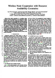
where  > 0 is arbitrarily small. Moreover, the achievable throughput of the cache-assisted multihop scheme RM satisfies the same scaling law as that of RP HY , i.e., RM = Θ (RP HY ). For the special case of Regime I or Regime II with α ≥ 3, Theorem 4 reduces to the achievable scaling law of the two baseline schemes in Theorem 5. In Regime II with α < 3, the scaling law achieved by the cache-induced hierarchical cooperation in Theorem 4 is better than that achieved by the two baseline schemes. As shown in Fig. 9, the achievable scaling laws of all schemes exhibit some phase transition phenomena as the content popularity skewness τ increases. Specifically, in Regime II, there are two critical popularity skewness points: τ = τa and τ = τb , where τa = 1, τb = 1.5 for the baseline schemes and τa = 1, τb =

min(3,α) 2

for the cache-induced hierarchical cooperation scheme. For the sub-critical case when

2

Achievable per node throughput scaling laws

10

"Proposed" "Baselines" 1

Super−critical case for proposed (τ > α/2): Caching provides a large order gain

10

0

Sub−critical case for proposed (τ < 1): Caching does not provide order gain

10

Super−critical case for baselines (τ > 1.5)

−1

10

Sub−critical case for baselines (τ < 1) −2

10

0

0.5

1 1.5 Content popularity skewness τ

2

Figure 9: Illustration of achievable throughput scaling laws in Theorem 4 for cache-induced hierarchical cooperation (solid curve) and Theorem 5 for baseline schemes (dashed curve). The number of nodes in the extended network is n = 411 . The total content size order β1 = 0.9 and the cache size order is β2 = 0.3 (i.e., Regime II). The path loss exponent is α = 2.5. In the figure, the circle and star symbols indicate the first and second critical popularity skewness points τa and τb , respectively.

τ < τa , the per node throughput scales with n as Ω (nηa ) with a smaller order ηa . For example, when

for the cache-induced hierarchical cooperation, which is the β1 −β2 = 1 (i.e., LC  L), ηa = 1− min(3,α) 2 same as the scaling law of the hierarchical cooperation without caching; and ηa = −0.5 for the baseline schemes, which is the same as the Gupta–Kumar law [8]. Therefore, when τ < τa and β1 − β2 = 1, caching does not provide order gain. For the super-critical case when τ > τb , on the other hand, the per node throughput scales with n as Ω (nηb ) with a much larger order ηb . For example, when β1 − β2 = 1 (i.e., LC  L), we still have ηb = β2 (τ − 1) > 0 for all schemes. In this case, caching provides a large order gain even when LC  L. From Fig. 9, there are two advantages of the proposed cache-induced hierarchical cooperation over the PHY caching. First, when α < 3, the second critical popularity skewness point τb of the cache-induced hierarchical cooperation is smaller than that of the baseline schemes. This implies that the cache-induced hierarchical cooperation can enjoy the large order gain ηb = β2 (τ − 1) under weaker conditions on the popularity distribution. Second, when α < 3, the cache-induced hierarchical cooperation can achieve a better scaling law for τ < 1.5.

C. Main Converse Results In this section, we establish upper bounds on the throughput scaling laws. The main converse results are summarized in the following theorem. Theorem 6 (Upper Bound of Scaling Laws in Extended Networks). In an extended wireless D2D caching network, the per node throughput R of any feasible content delivery scheme must satisfy the following scaling laws. In Regime I, we have R=

  O (n ) ,

τ ∈ [0, 1]

 O nβ2 (τ −1)+
,

τ >1

.

In Regime II, we have     −1)+ (β2 −β1 )( min(3,α)  2  , O n      min(3,α) min(3,α) R = O nβ1 (τ − 2 )+β2 ( 2 −1)+ ,    
  O nβ2 (τ −1)+ ,

τ ∈ [0, 1]  i , τ ∈ 1, min(3,α) 2 τ>

min(3,α) 2

where  > 0 is arbitrarily small. Please refer to Section VII-D for the proof. In both Regime I and Regime II, the multiplicative gap between the achievable per node throughput in Theorem 4 and its upper bound in Theorem 6 is within n for  > 0 that can be arbitrarily small as n → ∞. Therefore, the throughput scaling law depicted in Theorem 4 is order-optimal in the information

theoretic sense for the Zipf popularity distribution.

D. Converse Proof 1) Regime II with τ >

min(3,α) : 2

The converse result for this case can be proved by considering the

cut set bound between a reference node i and the rest of the network as follows. Let ql = I (Bi ; Wl ) /F .

Since Bi is a function of W1 , ..., WL , we have H (Bi ) = H (Bi ) − H (Bi |W1 , ..., WL ) = I (Bi ; W1 , ..., WL ) a

=

L X

I (Bi ; Wl |W1 , ..., Wl−1 )

l=1 b

=

L X

I (Bi , W1 , ..., Wl−1 ; Wl )

l=1

≥

L X

I (Bi ; Wl ) =

l=1

L X

ql F,

(15)

l=1

where (15-a) follows from the chain rule and (15-b) follows from the fact that the messages W1 , ..., WL are P mutually independent. Hence, the ql ’s must satisfy the cache capacity constraint L l=1 ql F ≤ H (Bi ) ≤ LC F .

Under any feasible content delivery scheme, the amount of information uji transmitted from the rest h i of the network to node i during the time window tji , ..., tj+1 − 1 must satisfy i   uji ≥ H Uij |Bi (16)     = H Wli , Uij |Bi − H Wli |Uij , Bi ≥ H (Wli |Bi ) − εF F

(17)

= H (Wli ) − I (Wli ; Bi ) − εF F = F (1 − qli − εF ) ,

where εF → 0 as F → ∞, (16) is to ensure that node i can successfully receive the aggregate information message Uij , and (17) follows from the necessary condition in (1). As a result, for given ql ’s and per node rate requirement R, the total average traffic rate over the cut from the rest of the network to node P  L i is p (1 − q ) − ε R. Clearly, a per node throughput R is achievable only if the induced total F l l l=1 average traffic rate does not exceed the sum capacity Γi of the MISO channel between the rest of the network and node i, which is upper bounded by K log n for some constant K [12]. Hence, the achievable per node throughput is upper bounded by R ≤ max PL {ql }

l=1 pl

Γi (1 − ql ) − εF

, s.t.

L X

ql ≤ dLC e .

l=1

It is easy to see that the optimal ql ’s to maximize the achievable per node throughput upper bound is to cache the most popular dLC e files, i.e., ql? = 1, l = 1, ..., dLC e and ql? = 0, l > dLC e. As a result, we

Figure 10: Illustration of reference square to construct the cut set bound in Lemma 4.

have R ≤ PL

Γi

l=1 pl

In Regime II with τ >

min(3,α) , 2


?

1 − ql − ε F

= PL

Γi

? l=dLC e+1 pl

− εF

.

(18)

we have L X

  p?l = Ω nβ2 (1−τ ) .

(19)

l=dLC e+1


Finally, it follows from Γi ≤ K log n, (18), and (19) that R = O nβ2 (τ −1)+ as F → ∞. h i 2) Regime II with τ ∈ 0, min(3,α) or Regime I: Draw a reference square at the center of the network 2 q β −β 1 2 with side length 12 n 2 , as illustrated in Fig. 10. Let Sc denote the set of nodes outside the reference square and Dc denote the set of nodes inside the reference square. The converse result for this case can be proved by considering the cut set bound between Sc and Dc as follows. Let ql = I (∪i∈Dc Bi ; Wl ) /F . Following similar analysis to that in Section VII-D1, the ql ’s must satisfy the total cache capacity P 1 β1 −β2 constraint L . Moreover, under any feasible content delivery l=1 ql ≤ |Dc | LC , where |Dc | = 2 n scheme, the amount of information uji transmitted from the nodes in Sc to node i during the time h i window tji , ..., tj+1 − 1 must satisfy uji ≥ (1 − qli − εF ) F . As a result, for given ql ’s and per node rate i P  L requirement R, the total average traffic rate over the cut from Sc to Dc is |Dc | p (1 − q ) − ε R. F l l l=1 Clearly, a per node throughput R is achievable only if the induced total average traffic rate does not exceed the sum capacity Γc of the MIMO channel between the Sc and Dc . Hence, the achievable per

node throughput is upper bounded by Γc

R ≤ max {ql }

|Dc |

P

L l=1 pl

(1 − ql ) − εF

 , s.t.

L X

ql ≤ d|Dc | LC e .

l=1

It is easy to see that the optimal ql ’s to maximize the achievable per node throughput upper bound is to cache the most popular d|Dc | LC e files, i.e., ql? = 1, l = 1, ..., d|Dc | LC e and ql? = 0, l > d|Dc | LC e. As a result, we have R≤

where pc ,

PL

l=1 pl

(1 − ql? ) =

Γc , pc |Dc |

(20)

PL

l=d|Dc |LC e+1 pl

satisfies     Ω (1) , τ ∈ [0, 1)      . pc = Ω 1 τ =1 log n    
 Ω nβ1 (1−τ ) , τ > 1

The following lemma bounds the sum capacity Γc between the Sc and Dc . Lemma 4. The sum capacity Γc of the MIMO channel between the Sc and Dc is bounded as   min(3,α) Γc ≤ Θ n(β1 −β2 )(2− 2 )+ ,

(21)

where  < 0 is arbitrarily small. Please refer to Appendix E for the proof. Substituting the upper bound of Γc in (21) into (20) and letting F → ∞, we obtain the desired results h i in Theorem 6 for Regime II with τ ∈ 0, min(3,α) as well as Regime I. 2 VIII. C ONCLUSION In this paper, we combine wireless device caching and hierarchical cooperation to significantly improve the capacity of wireless D2D networks. Specifically, we propose a cache-induced hierarchical cooperation scheme where the network is abstracted as a tree graph with each virtual node in the graph representing a cluster of nodes in the network, and the content files are cached at different levels of the tree graph according to their popularities. The PHY has two possible modes: hierarchical cooperation mode or multihop mode, depending on which mode yields a better throughput. The corresponding optimal cache content placement is formulated as an integer programming problem. We propose a low-complexity cache content placement algorithm to solve the integer programming problem and bound the gap w.r.t. the optimal solution. Then we analyze the throughput performance of the cache-induced hierarchical

cooperation scheme and show that the proposed scheme achieves significant throughput gain over the cache-assisted multihop scheme, which only supports multihop mode in the PHY. Finally, for extended networks under Zipf popularity distribution, we establish the per node capacity scaling law by showing that the multiplicative gap between the achievable per node throughput of the cache-induced hierarchical cooperation and an upper bound of the per-node throughput is within n for  > 0 that can be arbitrarily small. When the path loss exponent α < 3, the optimal per-node capacity scaling law in this paper can be significantly better than that achieved by the existing state-of-the-art schemes. To the best of our knowledge, this is the first work that completely characterizes the per-node capacity scaling law for wireless caching networks under the physical model and Zipf distribution. For clarity, we have assumed an independent phase fading channel model. However, the achievable throughput analysis in Theorem 3, and the capacity scaling law for extended networks in Theorem 4 and 6 can be readily extended to the more general PHY model. For an arbitrary PHY model, Theorem 3 and 6 still hold if we replace the coefficients cn and γn in Theorem 3 (achievable throughput bounds) and the cut set bounds of the sum capacities Γi and Γc in the converse proof in Section VII-D with proper expressions under the specific PHY model. For example, for an extended network under the free √  propagation model with α = 2, the results in [32] show that γn = 1 − log λn / log n, Γi = O (log n)  √   β1 −β2 n and Γc = Θ as n → ∞, and thus the capacity scaling law in Regime II is given by λ    β −β  β2 −β1 n 2 2 1   τ ∈ [0, 1] Θ λ       i β 3 min(3,α) . R = Θ λβ2 −β1 nβ1 (τ − 2 )+ 22 τ ∈ 1, 2    
 Θ nβ2 (τ −1) , τ > min(3,α) 2 In Regime I, the capacity scaling law is still given by Theorem 4 and 6. A PPENDIX A. Proof of Theorem 2 First, we show that if (x∗ , R∗ ) is the optimal solution of Problem (8), it must satisfy the conditions in Theorem 2. The conditions R ≤ C m∗ and (10-11) are the constraints in Problem (8). Therefore, we only 0

need to prove that (x∗ , R∗ ) satisfy the first condition in (9). Suppose there exist m ∈ {m∗ + 1, ..., M } P 0  m −1 ∗ such that f x + 1 R∗ < C m0 . Then we can find another feasible solution x to strictly i=m∗ i improve the objective function R as follows. Let xm0 = x∗m0 + ε, where ε > 0 is a sufficiently  0 0 0 small number. Let xm0 −1 = x∗m0 −1 − ε, xi = x∗i − ε , ∀i ∈ / {0, 1, ..., m∗ − 1} ∪ m − 1, m , and

x0 = x0 +

0

P

∗ −1}∪ m0 −1,m0 i∈{0,1,...,m / { }ε , Pm−1 be verified that i=m∗ xi >

0

where ε > 0 is a sufficiently small number compared  Pm−1 ∗ Pm0 −1 ∗ , ..., M } \ m0 x , ∀m ∈ {m and ∗ i i=m i=m∗ xi >

to ε. It can Pm0 −1 ∗ i=m∗ xi −ε. Since f (x) is a strictly decreasing function of x with a bounded derivative, for sufficiently P  P  0 m−1 m−1 ∗ ∗ < f small ε, we have f x + 1 R x + 1 R∗ ≤ C m , ∀m ∈ {m∗ , ..., M } \m and ∗ ∗ i i i=m i=m P 0  P 0  m −1 m −1 ∗ < f f x + 1 R x + 1 − ε R∗ < C m0 . Therefore, we can strictly increase R ∗ ∗ i i i=m i=m

without violating any constraints. Hence, at the optimal solution (x∗ , R∗ ), the condition in (9) must be satisfied. In the following, we show that the solution to the conditions in Theorem 2 is unique, which implies that these conditions are also sufficient for (x∗ , R∗ ) to be the optimal solution of Problem (8). Specifically, it can be shown that


Lm C m > Lm C m+1 = Lm+1 C m+1


Lm C m = Lm−1 C m < Lm−2 C m−1 .

(22)



If m∗ is the solution to the optimality conditions, we must have Lm∗ C m∗ +1 < LC and Lm∗ C m∗ ≥

LC . Then it follows from (22) that Lm C m < LC , ∀m > m∗ and Lm C m+1 ≥ LC , ∀m < m∗ ,

which implies any m 6= m∗ cannot satisfy the two conditions Lm C m+1 < LC and Lm C m ≥ LC simultaneously. Therefore, the solution to the conditions in Theorem 2 is unique.

B. Reformulation of the Problem (3) We reformulate Problem (3) as a ZOLP for fixed R as follows. Define the binary variables δm,l ∈ {0, 1} and the (M + 2) × L matrix 4 = [δm,l ] formed as follows: the first row is the all-one vector, that is, δm,l = 1 for all l = 1, . . . , L. The last row is the all-zero vector, that is, δM +1,l = 0 for all l = 1, . . . , L.

The remaining rows between m = 1 and m = M satisfy the following monotonicity conditions on the rows and on the columns: δm,l ≤ δm,l+1 , m = 1, ..., M, l = 1, ..., L, δm,l ≥ δm+1,l , m = 1, ..., M, l = 1, ..., L.

In words, the matrix 4 has monotonically non-decreasing rows, and monotonically non-increasing columns. Since the δ -variables are binary, this means that each row of 4 is formed by a leading block of zeros followed by a block of ones, and each column of 4 is formed by a leading block of ones followed by a block of zeros.

Observation 1: For m = 0, . . . , M , we let xm =

L X

δm,l −

l=1

L X

δm+1,l .

l=1

Hence, the link capacity constraint (4) can be written as a linear constraint with respect to the variables δm,l for fixed R as follows 4pR ≤ c,

where p is the L × 1 vectors containing the file request distribution {pl }, and c is a (M + 2) × 1 vector with the first element c0 = R, the last element cM +1 = 0, and elements m = 1, . . . , M equal to cm = Cm 4−(m−1) .

Observation 2: We define row-differential matrix of dimensions (M + 1) × (M + 2) given by   1 −1 0 · · · 0      0 1 −1 0 · · · 0    ..   .. . . . . D= . . . . .       0 ··· 0 1 −1 0    0 ··· 0 1 −1 Then, it is not difficult to see that the cache size constraint (5) can be rewritten as wT D41 ≤ LC ,

where w is a (M + 1) × 1 weight vector with elements wm = 4−m and 1 is the all-one column vector of dimension L × 1. Observation 3: The constraint (6) with this new parameterization of the problem becomes irrelevant since it is automatically imposed by the side of the matrix 4. It follows that the problem re-parameterized in the binary variables δm,l can be written as max R R,4

s.t. 4pR ≤ c, wT D41 ≤ LC , δm,l ≤ δm,l+1 , m = 1, ..., M, l = 1, ..., L, δm,l ≥ δm+1,l , m = 1, ..., M, l = 1, ..., L, δ0,l = 1, l = 1, ..., L, δm+1,l = 0, l = 1, ..., L.

(23)

This is a ZOLP feasibility problem for any fixed value of R. Therefore, it is possible to use standard ZOLP solvers for fixed R, and perform a bisection search over R ∈ [0, Rmax ], where Rmax is some upper bound on the per node throughput that can be found by, e.g., relaxing the binary constraint on δm,l to δm,l ∈ [0, 1].

C. Proof of Lemma 3 After steps 2a and 2b of Algorithm 1, at the m∗ level, we have xom∗ = bx∗m∗ c < x∗m∗ , and thus M X

x◦i =

i=m∗ M X

M X

x∗i = L,

i=m∗

x◦i

=L−

bx∗m∗ c


x∗m∗+1 + 4 (x∗m∗ − xom∗ ) , and thus

  x◦i = L − x∗m∗+1 + 4 (x∗m∗ − xom∗ ) − bx∗m∗ c

i=m∗ +2 M X


0 and

and thus

◦ m −1 X

R∗ = C m◦ /f

! x∗i + 1

≤ C m◦ /f (2) .

(25)

i=m∗

There are three cases as follows: Case 1: M ◦ − m◦ = 0: In this case, the achievable throughput after steps 2a and 2b is R◦ = C M ◦ /f (1) .

It follows from (24) that

PM

i=M ◦

x∗i >

PM

x◦i − 1 = L − 1, and thus ! ◦ M −1 X x∗i + 1 ≤ C M ◦ /f (2) .

i=M ◦

R∗ = C M ◦ /f

i=m∗

Therefore, R◦ /R∗ = f (2) /f (1) ≥ 1/ (1 + 2τ ) .

(26)

Case 2: M ◦ − m◦ = 1: In this case, the achievable throughput after steps 2a and 2b is ! ◦ ◦ C C m m +1
R◦ = min , Pm◦ ◦ f (1) f i=m∗ xi + 1 ≥

C m◦ +1 . f (1)

(27)

From (25), we have C m◦ f (2) ≥ ≥ 1/ (1 + 2τ ) . ∗ f (1) R f (1)

If x◦m◦ < L − 1, we have

Pm◦

x◦i + 2 ≤ L, and thus P ◦  m ∗+1 f x i=m∗ i C m◦ +1

= Pm◦ P ◦ m ◦ ◦ ∗ f f i=m∗ xi + 1 R i=m∗ xi + 1 P ◦  m ◦+2 f x ∗ i i=m 1
≥ . ≥ Pm◦ ◦ 1 + 2τ f i=m∗ xi + 1 i=m∗

If x◦m◦ = L − 1, C m◦ +1 1 f (2)
≥ , = Pm◦ ◦ ∗ 4f (L) 1 + 2τ f i=m∗ xi + 1 R

for L ≥ 2. From the above analysis, we have 1 R◦ /R∗ = f (2) /f (1) ≥ 1/ (1 + 2τ ) . 4

(28)

Case 3: M ◦ − m◦ > 1: In this case, after Step 2f is performed for the first time, the achievable 0

throughput under the cache content placement parameter x is given by   C 0 m  . R = ◦ min ◦  P m−1 0 m ≤m≤M f i=m∗ xi + 1 If x◦M ◦ < 3, we have x◦M ◦ = 0, and thus

C ◦ P ◦M −1 0 f( M i=m∗ xi +1)

CM◦ f

P

M ◦ −1 0 i=m∗ xi



+ 1 R∗

=

CM◦ f (L+1)

= +∞. Otherwise, x◦M ◦ ≥ 3 and

CM◦

≥

 + 1 R∗ P ◦  M −1 ∗ f x + 1 ∗ i i=m  = P ◦ M −1 ◦ f x + 1 i=m∗ i f

≥

P

M ◦ −1 ◦ i=m∗ xi

f (L − x◦M ◦ + 2) 1
≥ . 1 + 2τ f L − x◦M ◦ + 1

(29)

For m = m◦ + 1, we have C m◦ +1 C m◦ +1

= Pm◦ Pm◦ 0 ◦ ∗ ∗ f f i=m∗ xi + 1 R i=m∗ xi R P ◦  m ∗+1 f x ∗ i i=m
= Pm◦ ◦ f i=m∗ xi P ◦  m ◦ f i=m∗ xi + 2 1
≥ . ≥ Pm◦ ◦ 1 + 2τ f i=m∗ xi

(30)

Similarly, it can be shown that 1 C P m > , m = m◦ , ..., M ◦ , τ 0 m−1 1 + 2 f i=m∗ xi + 1 0

from which it follows that R /R∗ ≥

1 1+2τ .

Since steps 2c to 2g do not decrease the achievable throughput, it follows from the above analysis that R◦ /R∗ ≥ 1/ (1 + 2τ ) also holds after the termination of the algorithm. Finally, the additional factor of 1 M

is because

1 (m−1) M C m4

≤ Cm ≤ C m 4(m−1) and we have used the upper bound C m 4(m−1) in the

relaxed cache content placement optimization problem in (8).

D. Proof of Theorem 3 We first give some useful lemmas. The following lemma follows immediately from the optimality condition in Theorem 2.  Lemma 5. Let 0 ≤ f L (R, m∗ ) ≤ Lm∗ (R) , R ∈ C m∗ +1 , C m∗ and f U (R, m∗ ) ≥ Lm∗ (R) , R ∈  C m∗ +1 , C m∗ be some lower bound and upper bound of Lm∗ (R), respectively. For any RU that satisfies  f L (RU , m∗ ) ≥ LC , RU ∈ C m∗ +1 , C m∗ for some m∗ ∈ Z+ , we have RU ≥ R∗ , where R∗ is the optimal solution of the relaxed cache content placement optimization problem in (8). And for any RL that satisfies  f U (RL , m∗ ) ≤ LC , RL ∈ C m∗ +1 , C m∗ for some m∗ ∈ Z+ , we have RL ≤ R∗ . The following lemma gives closed-form bounds for f −1



Cm R



.

Lemma 6. For different regions of τ , f −1 f

−1

f

−1

f

−1

 



Cm R



Cm R



Cm R



 ≥



Cm R

can be lower bounded as

Cm 1− (1 − τ ) R

≥ e−1 L1− ≥2



1−τ

Cm R

+ , τ ∈ [0, 1)

,τ = 1

 min

C mτ R

1  1−τ

! , L + 1 , τ > 1.

and upper bounded as f

−1

f

−1

f

−1



Cm R





Cm R





Cm R



≤1−

Cm , τ ∈ [0, 1) R

≤ e2 L, τ = 1

 ≤ min

Cm τR

1  1−τ

! ,L + 1

Proof: The upper bound follows from the fact that f (x) ≥ R L+1

from the fact that f (x) ≤

z −τ dz+bxc R L+1 z −τ dz 1

bxc

−1

+ 1, τ > 1.

R L+1 −τ z dz R xL z −τ dz+1 1

and the lower bound follows

. The detailed calculations are omitted for conciseness.

With the above lemmas, we are ready to prove Theorem 3. The proof contains five cases depending on the value of τ .   Case 1: τ ∈ [0, 1): We first prove the lower bound. Replace f −1 CRm in Lm∗ (R) with the upper   bound of f −1 CRm for τ ∈ [0, 1) in Lemma 6, and we obtain an upper bound of Lm∗ (R) as   ∗ 3cn 4γn +1 4−γn (m +1) ∗ ∗ f U (R, m ) = L 4 − 4−(m +1) . γ +1 n R (4 − 1) γn

3cn a , m∗ ) ≤ a and m∗ = 0 satisfies f U (RL > 1 − 4γ3·4 L n +1 −1 , it can be verified that RL = (4γn +1 −1)(1− LC )  a ∈ C ∗ , C ∗ . On the other hand, if LC ≤ 1 − 3·4γn , it can be verified that Rb = LC , RL m +1 m L 4γn +1 −1  −γn j kL

 γ LC n cn 12 1 ∗ b ∗ b cn 4 − 4γn +1 −1 and m = γn log4 RL satisfies f U RL , m ≤ LC , RL ∈ C m∗ +1 , C m∗ . L

If

LC L

Then from Lemma 5, the lower bound given in Theorem 3 is valid for τ ∈ [0, 1).     Then we prove the upper bound. Replace f −1 CRm in Lm∗ (R) with the lower bound of f −1 CRm for τ ∈ [0, 1) in Lemma 6, and we obtain a lower bound of Lm∗ (R) as  1   1 3 · 4γn R γn ∗ f L (R, m ) = L 1 − γn +1 (1 − τ ) γn cn (4 − 1)    1 1 3 · 4γn R γn γ ≥ L 1 − γn +1 (1 − τ ) n , (4 − 1) cn

∗

where the last inequality follows from 4−m < 4 LC , and we have RU =

Clearly, the above RU and m∗ =

j

cn 1−τ 1 γn



log4

1−

  R cn

 since R > C m∗ +1 . Let L 1 −

3 · 4γn (4γn +1 − 1)

k+

cn RU

1 γn

−γn 

LC L

3·4γn (4γn +1 −1)



1

(1 − τ ) γn

γn .

 satisfy f L (RU , m∗ ) > LC , RU ∈ C m∗ +1 , C m∗ . Then

from Lemma 5, the upper bound RU given in Theorem 3 is valid for τ ∈ [0, 1).   Case 2: τ = 1: We first prove the lower bound. Replace f −1 CRm in Lm∗ (R) with the upper bound   of f −1 CRm for τ = 1 in Lemma 6, and we obtain an upper bound of Lm∗ (R) as

∗ f U (R, m∗ ) = e2 L − 1 4−m − e2 L − L − 1 4−M  1

R γn 2 ≤ e L−1 4 − e2 L − L − 1 4−M , cn  1
  γ1
∗ γ where the last inequality follows from 4−m < 4 cRn n . Let e2 L − 1 4 RcnL n − e2 L − L − 1 4−M = LC , and we have

!γn
e2 L − L − 1 4−M + LC RL = cn . 4 (e2 L − 1) j k+  Clearly, the above RL and m∗ = γ1n log4 RcnL satisfy f U (RL , m∗ ) ≤ LC , RL ∈ C m∗ +1 , C m∗ . Then 1 M (1+2τ ) RL

given in Theorem 3 is valid for τ = 1.     Then we prove the upper bound. Replace f −1 CRm in Lm∗ (R) with the lower bound of f −1 CRm

from Lemma 5, the lower bound

for τ = 1 in Lemma 6, and we obtain a lower bound of Lm∗ (R) as M X

3L f L (R, m ) = e ∗

cn

∗

m=m +1



3L ≥ e

where the last inequality follows from

R cn cn R



1 γn

−mγn

L− R 4 4m M −m X

− (L + 1) 4−M −γn (m−1)

4−m L−4

− (L + 1) 4−M ,


LC , RU ∈ C m∗ +1 , C m∗ . Then Clearly, the above RU and m∗ = γ1n log4 RcnU

Let

3L e

RU cn

4

from Lemma 5, the upper bound RU given in Theorem 3 is valid for τ = 1.



RU cn



1 γn

=

  Case 3: τ ∈ (1, γn + 1): We first prove the lower bound. Replace f −1 CRm in Lm∗ (R) with the   upper bound of f −1 CRm for τ > 1 in Lemma 6, and we obtain an upper bound of Lm∗ (R) as  f U (R, m∗ ) =

4

 1+γn −τ   1 τ R γn − 4 L γn cn  1+γn −τ  . 4 τ −1 − 1

γn +τ −1 τ −1

Let f U (RL , m∗ ) = LC , and we have !γn 1+γn −τ cn 4 τ −1 − 1 RL = LγCn Lτ −1−γn . γn +τ −1 τ 4 τ −1 − 4 k+ j  satisfy f U (RL , m∗ ) ≤ LC , RL ∈ C m∗ +1 , C m∗ . Then Clearly, the above RL and m∗ = γ1n log4 RcnL 1 M (1+2τ ) RL

given in Theorem 3 is valid for τ ∈ (1, γn + 1).     Then we prove the upper bound. Replace f −1 CRm in Lm∗ (R) with the lower bound of f −1 CRm

from Lemma 5, the lower bound

for τ > 1 in Lemma 6, and we obtain a lower bound of Lm∗ (R) as  1 1+γn −τ τ R γn L γn cn ∗ f L (R, m∗ ) = − 4−m τ −1 2  1 1+γn −τ τ R γn  1 L γn cn R γn ≥ , − 4 2τ −1 cn where the last inequality follows from  1 γ 4 RcnU n = LC , and we have

∗ 4−m



L RU = LγCn  Clearly, the above RU and m∗ =

j

1 γn

log4

< 4

1+γn −τ γn

cn RU

  R cn

  τ cn

1 γn

1+γn −τ γn



τ RU cn τ −1

2



1 γn

−

−γn

1 γn

2τ −1

k+

since R > C m∗ +1 . Let

L

−

− 4cn

1 γn

.

 

 satisfy f L (RU , m∗ ) > LC , RU ∈ C m∗ +1 , C m∗ . Then

from Lemma 5, the upper bound RU given in Theorem 3 is valid for τ ∈ (1, γn + 1).     Case 4: τ = γn + 1: Replace f −1 CRm in Lm∗ (R) with the upper bound of f −1 CRm for τ > 1 in Lemma 6, and we obtain an upper bound of Lm∗ (R) as ∗

f U (R, m ) = (3 log4 L + 4)



τR cn



Let f U (RL , m∗ ) = LC , and we have RL = (3 log4 L + 4)−γn

cn γn L . τ C

1 γn

.

Clearly, the above RL and m∗ =

j

from Lemma 5, the lower bound

1 M (1+2τ ) RL

1 γn

log4

cn RL

k+

 satisfy f U (RL , m∗ ) ≤ LC , RL ∈ C m∗ +1 , C m∗ . Then

given in Theorem 3 is valid for τ = γn + 1.

For the throughput upper bound, consider a scheme which caches the most popular LC files at the 0-th level and the remaining L − LC files at the 1-th level. Clearly, the throughput achieved by such a

scheme must be larger than R∗ and is given by
τ − L1−τ cn 4−γn cn 4−γn ≤ . f (L − LC + 1) (LC + 1)1−τ − (L + 1)1−τ     Case 5: τ > γn + 1: Replace f −1 CRm in Lm∗ (R) with the upper bound of f −1 CRm for τ > 1 in Lemma 6, and we obtain an upper bound of Lm∗ (R) for R ≤ cn Lτ −1 as !  1 γn +1−τ 1 1 3τ τ −1 4 τ −1 R τ −1 ∗ f U (R, m ) = . + 4τ γn γn +1−τ cn 1 − 4 τ −1 Let f U (RL , m∗ ) = LC , and we have 1

RL = cn

Clearly, the above RL and m∗ =

j

1 γn

3τ τ −1 4

log4

γn +1−τ τ −1

1−4 k+ cn RL

RL ≤ cn Lτ −1 , from Lemma 5, the lower bound

!1−τ

γn +1−τ τ −1

+ 4τ

1 γn

LτC−1 .

 satisfy f U (RL , m∗ ) ≤ LC , RL ∈ C m∗ +1 , C m∗ . Since 1 M (1+2τ ) RL

given in Theorem 3 is valid for τ > γn + 1.

The throughput upper bound is the same as in case 4. This completes the proof.

E. Proof of Lemma 4 Lemma 4 can be proved using similar a technique to that in the proof of Theorem 5.2 in [12]. With some bounded per node power constraint P , the sum capacity of the MIMO channel between the Sc and Dc is Γc =


max E log I + HQ (H) H H , Q (H)  0
E Qj,j (H) ≤ P, ∀j ∈ Sc

(33)

where H = [hi,j ]i∈Dc ,,j∈Sc . Let V c denote the set of nodes inside the square at the center of the
2 √ network with area nc − 2 , where nc = nβ1 −β2 , and let Vc = Dc \V c . By the generalized Hadamard’s inequality, we have log I + HQ (H) H H ≤ log I + H (1) Q (H) H (1)H + log I + H (2) Q (H) H (2)H ,

where H (1) = [hi,j ]i∈Vc ,,j∈Sc is the channel between the Sc and Vc , and H (2) = [hi,j ]i∈V c ,,j∈Sc is the channel between the Sc and V c , and thus (33) is bounded above by     (1) (1) (1)H Γc ≤ max E log I + H Q H H   (1) Q H 0    E Qj,j H (1) ≤ P, ∀j ∈ Sc     (2) (2) (2)H + max E log I + H Q H H .   (2) Q H 0    E Qj,j H (2) ≤ P, ∀j ∈ Sc

(34)

Applying Hadamard’s inequality once more, the first term in (34) can be upper-bounded by the sum of the capacities of the individual MISO channels between nodes in Sc and each node in Vc . Following a similar analysis to that in the proof of Theorem 5.2 in [12], the first term in (34) is upper bounded by 0 0√ K nc (log n)2 , where K is a constant independent of n. To bound the second term in (34), we introduce the concept of the total power received by all the nodes in V c , when the nodes in Sc are transmitting independent signals with power P . Specifically, P −α . Let let Pj denote the total received power in V c of the signal sent by j ∈ Sc : Pj = P i∈V c ri,j  p  P P −α ˜ = hi,j / dj , where dj = i∈V c ri,j Ptot (nc ) = j∈Sc Pj and define H . Then the second i∈V c ,,j∈Sc term is equal to    H  ˜ ˜ ˜ H ˜ E log max I + H Q H   ˜ 0 Q H    ˜ j,j H ˜ E Q ≤ Pj , ∀j ∈ Sc    H  ˜ ˜ ˜ H ˜ E log I + H Q H ≤ max   ˜ 0 Q H     ˜ H ˜ E Tr Q ≤ Ptot (nc )    H  ˜ ˜ ˜ ˜ I + H Q H H 1 E log ≤ max Bn,   ˜ 0 Q H     ˜ H ˜ E Tr Q ≤ Ptot (nc )     H  ˜ ˜ ˜ ˜ c E Tr H Q H H 1Bn, , +  max  ˜ 0 Q H     ˜ H ˜ E Tr Q ≤ Ptot (nc )  

˜ 2 where the set Bn, = H

> n .

(35)

For the first term in (35), denoted as CBn, , using a similar analysis to Equation (11) in [12], it can be shown that   1 β1 −β2 nPtot (nc ) Pr (Bn, ) . ≤ n log 1 + 2 Pr (Bn, )

CBn,

(36)

Furthermore, following a similar analysis to Lemma 5.3 in [12], it can be shown that for any  > 0 and 0

p ≥ 1, there exists K1 > 0 such that for all n, 0

K Pr (Bn, ) ≤ p1 . n

(37)

It follows from (36), (37), and Ptot (nc ) ≤ P n2 that 0

CBn, ≤ K1 n

β1 −β2 −p

n3+p log 1 + 0 K1



 ,

(38)

which decays to zero with an arbitrary exponent as n tends to infinity. c , we have For the second term in (35), denoted as CBn,

c CBn, ≤

 max  ˜ 0 Q H     ˜ H ˜ E Tr Q ≤ Ptot (nc )

    

˜ 2 ˜ ˜ c E H Tr Q H 1Bn,

≤ n Ptot (nc ) .

(39)

Moreover, it can be verified that Ptot (nc ) =

  K 0 nc2−α/2 ,

α ∈ (2, 3)

 K 0 √nc ,

α≥3

.

(40)

Finally, (38-40) complete the Proof of Lemma 4. R EFERENCES [1] N. Golrezaei, K. Shanmugam, A. Dimakis, A. Molisch, and G. Caire, “Femtocaching: Wireless video content delivery through distributed caching helpers,” in Proc. IEEE INFOCOM, pp. 1107–1115, 2012. [2] M. Maddah-Ali and U. Niesen, “Fundamental limits of caching,” IEEE Trans. Info. Theory, vol. 60, no. 5, pp. 2856–2867, May 2014. [3] A. Liu and V. K. N. Lau, “Asymptotic scaling laws of wireless ad hoc network with physical layer caching,” IEEE Trans. Wireless Commun., vol. 15, no. 3, pp. 1657–1664, March 2016. [4] M. Ji, G. Caire, and A. Molisch, “Fundamental limits of distributed caching in D2D wireless networks,” 2013. [Online]. Available: http://arxiv.org/abs/1304.5856 [5] M. Ji, G. Caire, and A. F. Molisch, “The throughput-outage tradeoff of wireless one-hop caching networks,” IEEE Trans. Info. Theory, vol. 61, no. 12, pp. 6833–6859, Dec 2015.

[6] A. Altieri, P. Piantanida, L. R. Vega, and C. G. Galarza, “On fundamental trade-offs of device-to-device communications in large wireless networks,” IEEE Trans. Wireless Commun., vol. 14, no. 9, pp. 4958–4971, Sept 2015. [7] S.-W. Jeon, S.-N. Hong, M. Ji, and G. Caire, “Caching in wireless multihop device-to-device networks,” in Proc. IEEE ICC 2015, June 2015, pp. 6732–6737. [8] P. Gupta and P. Kumar, “The capacity of wireless networks,” IEEE Trans. Info. Theory, vol. 46, no. 2, pp. 388–404, Mar 2000. [9] X. Liang-Liang and P. R. Kumar, “A network information theory for wireless communication: scaling laws and optimal operation,” IEEE Trans. Info. Theory, vol. 50, no. 5, pp. 748–767, 2004. [10] A. Jovicic, P. Viswanath, and S. Kulkarni, “Upper bounds to transport capacity of wireless networks,” IEEE Trans. Info. Theory, vol. 50, no. 11, pp. 2555–2565, Nov 2004. [11] L.-L. Xie and P. Kumar, “On the path-loss attenuation regime for positive cost and linear scaling of transport capacity in wireless networks,” IEEE Trans. Info. Theory, vol. 52, no. 6, pp. 2313–2328, June 2006. [12] A. Ozgur, O. Leveque, and D. Tse, “Hierarchical cooperation achieves optimal capacity scaling in ad hoc networks,” IEEE Trans. Info. Theory, vol. 53, no. 10, pp. 3549–3572, Oct 2007. [13] U. Niesen, P. Gupta, and D. Shah, “On capacity scaling in arbitrary wireless networks,” IEEE Trans. Info. Theory, vol. 55, no. 9, pp. 3959–3982, Sept 2009. [14] ——, “The balanced unicast and multicast capacity regions of large wireless networks,” IEEE Trans. Info. Theory, vol. 56, no. 5, pp. 2249–2271, May 2010. [15] M. Franceschetti, M. D. Migliore, and P. Minero, “The capacity of wireless networks: Information-theoretic and physical limits,” IEEE Trans. Info. Theory, vol. 55, no. 8, pp. 3413–3424, Aug 2009. [16] S. N. Hong and G. Caire, “Beyond scaling laws: On the rate performance of dense device-to-device wireless networks,” IEEE Trans. Info. Theory, vol. 61, no. 9, pp. 4735–4750, Sept 2015. [17] S. Gitzenis, G. Paschos, and L. Tassiulas, “Asymptotic laws for joint content replication and delivery in wireless networks,” IEEE Trans. Info. Theory, vol. 59, no. 5, pp. 2760–2776, May 2013. [18] T. Yamakami, “A zipf-like distribution of popularity and hits in the mobile web pages with short life time,” in Proc. Parallel Distrib. Comput., Appl. Technol., Taipei, Taiwan, Dec 2006, pp. 240–243. [19] M. Ji, A. M. Tulino, J. Llorca, and G. Caire, “Caching and coded multicasting: Multiple groupcast index coding,” in proc. 2014 IEEE GlobalSIP, Dec 2014, pp. 881–885. [20] J. Hachem, N. Karamchandani, and S. Diggavi, “Multi-level coded caching,” in Proc. IEEE ISIT, Jun. 2014. [21] N. Karamchandani, U. Niesen, M. A. Maddah-Ali, and S. N. Diggavi, “Hierarchical coded caching,” IEEE Trans. Info. Theory, vol. 62, no. 6, pp. 3212–3229, June 2016. [22] A. Liu and V. Lau, “Cache-enabled opportunistic cooperative MIMO for video streaming in wireless systems,” IEEE Trans. Signal Processing, vol. 62, no. 2, pp. 390–402, Jan 2014. [23] ——, “Mixed-timescale precoding and cache control in cached MIMO interference network,” IEEE Trans. Signal Processing, vol. 61, no. 24, pp. 6320–6332, Dec 2013. [24] W. Han, A. Liu, and V. Lau, “Degrees of freedom in cached mimo relay networks,” IEEE Trans. Signal Processing, vol. 63, no. 15, pp. 3986–3997, Aug 2015. [25] W. Han, A. Liu, and V. K. N. Lau, “Improving the degrees of freedom in MIMO interference network via PHY caching,” in proc. 2015 IEEE GLOBECOM, Dec 2015, pp. 1–6.

[26] N. Naderializadeh, M. A. Maddah-Ali, and A. S. Avestimehr, “Fundamental limits of cache-aided interference management,” arXiv preprint arXiv:1602.04207, 2016. [27] J. Zhang and P. Elia, “Fundamental limits of cache-aided wireless BC: Interplay of coded-caching and CSIT feedback,” arXiv preprint arXiv:1511.03961, 2016. [28] A. Liu and V. K. N. Lau, “How much cache is needed to achieve linear capacity scaling in backhaul-limited dense wireless networks?” IEEE/ACM Transactions on Networking, vol. PP, no. 99, pp. 1–10, 2016. [29] A. Ozgur and O. Leveque, “Throughput-delay tradeoff for hierarchical cooperation in ad hoc wireless networks,” IEEE Trans. Info. Theory, vol. 56, no. 3, pp. 1369–1377, March 2010. [30] J. Ghaderi, L. L. Xie, and X. Shen, “Hierarchical cooperation in ad hoc networks: Optimal clustering and achievable throughput,” IEEE Transactions on Information Theory, vol. 55, no. 8, pp. 3425–3436, Aug 2009. [31] U. Niesen, D. Shah, and G. W. Wornell, “Caching in wireless networks,” IEEE Trans. Info. Theory, vol. 58, no. 10, pp. 6524–6540, Oct 2012. [32] S. H. Lee and S. Y. Chung, “Capacity scaling of wireless ad hoc networks: Shannon meets maxwell,” IEEE Trans. Info. Theory, vol. 58, no. 3, pp. 1702–1715, March 2012.