Multiscale Hierarchical Convolutional Networks - arXiv

Multiscale Hierarchical Convolutional Networks Jörn-Henrik Jacobsen 1 Edouard Oyallon 2 Stéphane Mallat 2 Arnold W.M. Smeulders 1

arXiv:1703.04140v1 [cs.LG] 12 Mar 2017

Abstract Deep neural network algorithms are difficult to analyze because they lack structure allowing to understand the properties of underlying transforms and invariants. Multiscale hierarchical convolutional networks are structured deep convolutional networks where layers are indexed by progressively higher dimensional attributes, which are learned from training data. Each new layer is computed with multidimensional convolutions along spatial and attribute variables. We introduce an efficient implementation of such networks where the dimensionality is progressively reduced by averaging intermediate layers along attribute indices. Hierarchical networks are tested on CIFAR image data bases where they obtain comparable precisions to state of the art networks, with much fewer parameters. We study some properties of the attributes learned from these databases.

1. Introduction Deep convolutional neural networks have demonstrated impressive performance for classification and regression tasks over a wide range of generic problems including images, audio signals, but also for game strategy, biological, medical, chemical and physics data (LeCun et al., 2015). However, their mathematical properties remain mysterious and we are currently not able to relate their performance to the properties of the classification problem. Classifying signals in high dimension requires to eliminate non-informative variables, and hence contract and reduce space dimensionality in appropriate directions. Convolutional Neural Networks (CNN) discover these directions via backpropagation algorithms (LeCun et al., 1989). Sev1

Informatics Institute, University of Amsterdam, Amsterdam Département Informatique, Ecole Normale Supérieure, Paris. Correspondence to: Jörn-Henrik Jacobsen . 2

Proceedings of the 34 th International Conference on Machine Learning, Sydney, Australia, 2017. JMLR: W&CP. Copyright 2017 by the author(s).

eral studies show numerically that linearization increases with depth (Zeiler & Fergus, 2014), but we do not know what type of information is preserved or eliminated. The variabilities which can be eliminated are mathematically defined as the group of symmetries of the classification function (Mallat, 2016). It is the group of transformations (not necessarily linear) which preserves the labels of the classification problem. Translations usually belong to the symmetry group, and invariants to translations are computed with spatial convolutions, followed by a final averaging. Understanding a deep neural network classifier requires specifying its symmetry group and invariants besides translations, especially of non-geometrical nature. To achieve this goal, we study highly structured multiscale hierarchical convolution networks introduced mathematically in (Mallat, 2016). Hierarchical networks give explicit information on invariants by disentangling, progressively more signal attributes as the depth increases. The deep network operators are multidimensional convolutions along attribute indices. Invariants are obtained by averaging network layers along these attributes. Such a deep network can thus be interpreted as a non-linear mapping of the classification symmetry group into a multidimensional translation group along attributes, which is commutative and hence flat. Signal classes are mapped into manifolds which are progressively more flat as depth increases. Section 2 reviews important properties of generic CNN architectures (LeCun et al., 2015). Section 3 describes multiscale hierarchical convolutional networks, which are particular CNNs where linear operators are multidimensional convolutions along progressively more attributes. Section 4 describes an efficient implementation, which reduces inner layers dimensions by computing invariants with an averaging along attributes. Numerical experiments on the CIFAR database show that this hierarchical network obtains comparable performances to state of the art CNN architectures, with a reduced number of parameters. Multiscale hierarchical network represent the symmetry group as multidimensional translations along non-linear attributes. Section 5 studies the structuration obtained by this deep network. This architecture provides a mathematical and experimental framework to understand deep neural network classification properties. The numerical results are reproducible

Multiscale Hierarchical Convolutional Networks

and code is available online using TensorFlow and Keras1 .

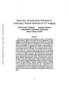
2. Deep Convolutional Networks and Group Invariants A classification problem associates a class y = f (x) to any vector x ∈ RN of N parameters. Deep convolutional networks transforms x into multiple layers xj of coefficients at depths j, whose dimensions are progressively reduced after a certain depth (LeCun et al., 2010). We briefly review their properties. We shall numerically concentrate on color images x(u, v) where u = (u1 , u2 ) are the spatial coordinates and 1 ≤ v ≤ 3 is the index of a color channel. The input x(u, v) may, however, correspond to any other type of signals. For sounds, u = u1 is time and v may be the index of audio channels recorded at different spatial locations. Each layer is an array of signals xj (u, v) where u is the native index of x, and v is a 1-dimensional channel parameter. A deep convolutional network iteratively computes xj+1 = ρ Wj+1 xj with x0 = x, as illustrated in Figure 1. Each Wj+1 computes sums over v of convolutions along u, with filters of small support. It usually also incorporates a batch normalization (Ioffe & Szegedy, 2015). The resolution of xj (u, v) along u is progressively reduced by a subsampling as j increases until an averaging in the final output layer. The operator ρ(z) is a pointwise non-linearity In this work, we shall use exponential linear units ELU (Clevert et al., 2015). It transforms each coefficient z(t) plus a bias c = z(t) + b into c if c < 0 and ec − 1 if c < 0. As the depth increases, the discriminative variations of x along u are progressively transferred to the channel index v. At the last layer xJ , v stands for the class index and u has disappeared. An estimation y˜ of the signal class y = f (x) is computed by applying a soft-max to xJ (v). It is difficult to understand the meaning of this channel index v whose size and properties changes with depth. It mixes multiple unknown signal attributes with an arbitrary ordering. Multiscale hierarchical convolution networks will adress this issue by imposing a high-dimensional hierarchical structure on v, with an ordering specified by the translation group. In standard CNN, each xj = Φj x is computed with a cascade of convolutions and non-linearities Φj = ρ Wj ... ρ W1 , whose supports along u increase with the depth j. These multiscale operators replace x by the variables xj to estimate the class y = f (x). To avoid errors, this change of variable must be discriminative, despite the dimensionality 1

https://github.com/jhjacobsen/HierarchicalCNN

reduction, in the sense that ∀(x, x0 ) ∈ R2N Φj (x) = Φj (x0 ) ⇒ f (x) = f (x0 ) . (1) This is necessary and sufficient to guarantee that there exists a classification function fj such that f = fj Φj and hence ∀x ∈ RN , fj (xj ) = f (x). The function f (x) can be characterized by its groups of symmetries. A group of symmetries of f is a group of operators g which transforms any x into x0 = g.x which belong to the same class: f (x) = f (g.x). The discriminative property (1) implies that if Φj (x) = Φj (g.x) then f (x) = f (g.x). The discrimination property (1) is thus equivalent to impose that groups of symmetries of Φj are groups of symmetries of f . Learning appropriate change of variables can thus be interpreted as learning progressively more symmetries of f (Mallat, 2016). The network must be sufficiently flexible to compute change of variables Φj whose symmetries approximate the symmetries of f . Deep convolutional networks are cascading convolutions along the spatial variable u so that Φj is covariant to spatial translations. If x is translated along u then xj = Φj x is alsoP translated along u. This covariance implies that for all v, u xj (u, v) is invariant to translations of x. Next section explains how to extend this property to higher dimensional attributes with multidimensional convolutions.

3. Multiscale Hierachical Convolution Networks Multiscale hierachical networks are highly structured convolutional networks defined in (Mallat, 2016). The onedimensional index v is replaced by a multidimensional vector of attributes v = (v1 , ..., vj ) and all linear operators Wj are convolutions over (u, v). We explain their construction and a specific architecture adapted to an efficient learning procedure. Each layer xj (u, v) is indexed by a vector of multidimensional parameters v = (v1 , ..., vj ) of dimension j. Each vk is an “attribute” of x which is learned to discriminate classes y = f (x). The operators Wj are defined as convolutions along a group which is a parallel transport in the index space (u, v). With no loss of generality, in this implementation, the transport is a multidimensional translation along (u, v). The operators Wj are therefore multidimensional convolutions, which are covariant to translations along (u, v). As previously explained, this covariance P to translations implies that the sum vk xj (u, v0 , ..., vj ) is invariant to translations of previous layers along vk . A convolution of z(u, v) by a filter w(u, v) of support S is written X z ? w(u, v) = z(u − u0 , v − v 0 ) w(u0 , v 0 ) . (2) (u0 ,v 0 )∈S


Figure 1. A deep convolution network compute each layer xj with a cascade of linear operators Wj and pointwise non-linearities ρ.

Since z(u, v) is defined in a finite domain of (u, v), boundary issues can be solved by extending z with zeros or as a periodic signal. We use zero-padding extensions for the next sections, except for the last section, where we use periodic convolutions. Both cases give similar accurcies. The network takes as input a color image x(u, v0 ), or any type of multichannel signal indexed by v0 . The first layer computes a sum of convolutions of x(u, v0 ) along u, with filters w1,v0 ,v1 (u) X x(·, v0 ) ? w1,v0 ,v1 (u) . (3) x1 (u, v1 ) = ρ

Proposition 3.1 The last layer xJ is invariant to translations of xj (u, v1 , ..., vj ) along (u, v1 , ..., vj ), for any j < J − 1. Proof: Observe that xJ = WJ ρ WJ−1 ...ρ Wj xj . Each Wk for j < k < J is a convolution along (u, v0 , ..., vj , ..., vk ) and hence covariant to translations of (u, v0 , ..., vj ). Since ρ is a pointwise operator, it is also covariant to translations. Translating xj along (u, v1 , ..., vj ) thus translates xJ−1 . Since (7) computes a sum over these indices, it is invariant to these translations.

v0

For any j ≥ 2, Wj computes convolutions of xj−1 (u, v) for v = (v1 , ..., vj−1 ) with a family of filters {wvj }vj indexed by the new attribute vj : xj (u, v, vj ) = ρ xj−1 ? wvj (u, v) . (4) As explained in (Mallat, 2016), Wj has two roles. First, these convolutions indexed by vj prepares the discriminability (1) of the next layer xj+1 , despite local or global summations along (u, v1 , ..., vj−1 ) implemented at this next layer. It thus propagates discriminative variations of xj−1 from (u, v1 , ..., vj−1 ) into vj . Second, each convolution with wvj computes local or global invariants by summations along (u, v1 , ..., vj−2 ), in order to reduce dimensionality. This dimensionality reduction is implemented by a subsampling of (u, v) at the output (4), which we omitted here for simplicity. Since vk is the index of multidimensional filters, a translation along vk is a shift along an ordered P set of multidimensional filters. For any k < j − 1, vk xj−1 (u, v1 , ..., vk , ..., vj−1 ) is invariant to any such shift. The final operator WJ computes invariants over u and all attributes vk but the last one: X xJ (vJ−1 ) = xJ−1 (u, v1 , ..., vJ−1 ) . (5) u,v1 ,...,vJ−1

The last attribute vJ−1 corresponds to the class index, and its size is the number of classes. The class y = f (x) is estimated by applying a soft-max operator on xJ (vJ−1 ).

This proposition proves that the soft-max of xJ approximates the classification function fj (xj ) = f (x) by an operator which is invariant to translations along the highdimensional index (u, v) = (u, v1 , ..., vj ). The change of variable xj thus aims at mapping the symmetry group of f into a high-dimensional translation group, which is a flat symmetry group with no curvature. It means that classes of xj where fj (xj ) is constant define surfaces which are progressively more flat as j increases. However, this requires an important word of caution. A translation of xj (u, v1 , ..., vj ) along u corresponds to a translation of x(u, v0 ) along u. On the contrary, a translation along the attributes (v1 , ..., vj ) usually does not correspond to transformations on x. Translations of xj along (v1 , ..., vj ) is a group of symmetries of fj but do not define transformations of x and hence do not correspond to a symmetry group of f . Next sections analyze the properties of translations along attributes computed numerically. Let us give examples over images or audio signals x(u) having a single channel. The first layer (3) computes convolutions along u: x1 (u, v1 ) = ρ(x ? wv1 (u)). For audio signals, u is time. This first layer usually computes a wavelet spectrogram, with wavelet filters wv1 indexed by a log-frequency index v1 . A frequency transposition corresponds to a log-frequency translation x1 (u, v1 − τ ) along v1 . If x is a sinusoidal wave then this translation corresponds to a shift of its frequency and hence to a transformation of x. However, for more general signals x, there exists no x0 such that ρ(x0 ? wv1 (u)) = x1 (u, v1 − τ ). It is indeed well known that a frequency transposition does not define


x(u, v0 ) ρW1

ρW2

ρW3

ρW4

ρW5

ρW6

ρW7

ρW8

ρW9

ρW10

ρW11

N2 × 3

x1 (u, v1 ) N2 × K

W12 xJ (vJ−1 ) 10/100

x2 (u, v1 , v2 )

x3 (u, v1 , v2 , v3 )

x5 (u, v3 , v4 , v5 )

x9 (u, v7 , v8 , v9 )

N2 × K × K

N2 × K × K ×K 4 2

× K × K ×K 4 2

× K × K ×K 4 2

N2 4

N2 16

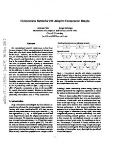
Figure 2. Implementation of a multiscale hierarchical convolutional network as a cascade of 5D convolutions Wj . The figure gives the size of the intermediate layers stored in 5D arrays. Dash dots lines indicate the parametrization of a layer xj and its dimension. We only represent dimensions when the output has a different size from the input.

an exact signal transformation. Other audio attributes such as timber are not either well defined transformations on x although important attributes to classify sounds. For images, u = (u1 , u2 ) is a spatial index. If wv1 = w(rv−1 u) is a rotation of a filter w(u) by an angle v1 then 1 x1 (u, v1 −τ ) = ρ(xτ ?wv1 (rτ u)) with xτ (u) = x(rτ−1 u). However, there exists no x0 such that ρ(x ? wv1 (u)) = x1 (u, v1 − τ ) because of the missing spatial rotation rτ u. These examples show that translation xj (u, v1 , .., vj ) along the attributes (v1 , ..., vj ) usually do not correspond to a transformation of x.

4. Fast Low-Dimensional Architecture 4.1. Dimensionality Reduction Multiscale hierarchical network layers are indexed by twodimensional spatial indices u = (u1 , u2 ) and progressively higher dimensional attributes v = (v1 , ..., vj ). To avoid computing high-dimensional vectors and convolutions, we introduce an image classification architecture which eliminates the dependency relatively to all attributes but the last three (vj−2 , vj−1 , vj ), for j > 2. Since u = (u1 , u2 ), all layers are stored in five dimensional arrays. The network takes as an input a color image x(u, v0 ), with three color channels 1 ≤ v0 ≤ 3 and u = (u1 , u2 ). Applying (3) and (4) up to j = 3 computes a fivedimensional layer x3 (u, v1 , v2 , v3 ). For j > 3, xj is computed as a linear combination of marginal sums of xj−1 along vj−3 . Thus, it does not depend anymore on vj−3 and can be stored in a five-dimensional array indexed by (u, vj−2 , vj−1 , vj ). This is done by convolving xj−1 with a a filter wvj which does not depend upon vj−3 : wvj (u, vj−3 , vj−2 , vj−1 ) = wvj (u, vj−2 , vj−1 ) .

(6)

We indeed verify that this convolution is a linear combination of sums over vj−3 , so xj depends only upon (u, vj−2 , vj−1 , vj ). The convolution is subsampled by 2sj with sj ∈ {0, 1} along u, and a factor 2 along vj−1 and vj xj (u, vj−2 , vj−1 , vj ) = xj−1 ? wvj (2sj u, 2vj−2 , 2vj−1 ) ,

At depth j, the array of attributes v = (vj−2 , vj−1 , vj ) is of size K/4 × K/2 × K. The parameters K and spatial subsmapling factors sj are adjusted with a trade-off between computations, memory and classification accuracy. The final layer is computed with a sum (7) over all parameters but the last one, which corresponds to the class index: X xJ (vJ−1 ) = xJ−1 (u, vJ−3 , vJ−2 , vJ−1 ) . u,vJ−3 ,vJ−2

(7) This architecture is illustrated in Figure 2. 4.2. Filter Factorization for Training Our newly introduced Multiscale Hierarchical Convolution Networks (HCNN) have been tested on CIFAR10 and CIFAR100 image databases. CIFAR10 has 10 classes, while CIFAR100 has 100 classes, which makes it more challenging. The train and test sets have 50k and 10k colored images of 32 × 32 pixels. Images are preprocessed via a standardization along the RGB channels. No whitening is applied as we did not observe any improvement. Our HCNN is trained in the same way as a classical CNN. We train it by minimizing a neg-log entropy loss, via SGD with momentum 0.9 for 240 epochs. An initial learning rate of 0.25 is chosen while being reduced by a factor 10 every 40 epochs. Each minibatch is of size 50. The learning is regularized by a weight decay of 2 10−4 (Krizhevsky et al., 2012). We incorporate a data augmentation with random translations of 6 pixels and flips (Krizhevsky & Hinton, 2010). Just as in any other CNNs, the gradient descent is badly conditioned because of the large number of parameters (Goodfellow et al., 2014). We precondition and regularize the 4 dimensional filters wvj , by normalizing a factorization of these filters. We factorize wvj (u, vj−3 , vj−2 , vj−1 ) into a sum of Q separable filters: wvj (u, vj−3 , vj−2 , vj−1 ) =

Q X

hj,q (u) gvj ,q (vj−2 , vj−1 ) ,

q=1

(8) and introduce an intermediate normalization before the sum. Let us write hj,q (u, v) = δ(u) hj,q (u) and


gvj ,q (u, v) = δ(u) gvj ,q (v). The batch normalization is applied to xj−1 ? hj,q and substracts a mean array mj,q while normalizing the standard deviations of all coefficients σj,q : x ˜j,q (u, v) =

xj−1 ? hj,q − mj,q . σj,q

This normalized output is retransformed according to (8) by a sum over q and a subsampling: xj (u, v) = ρ

Q X

x ˜j,q ? gvj ,q (2sj u, 2v) .

q=1

The convolution operator Wj is thus subdivided into a first operator Wjh which computes standardized convolutions along u cascaded with Wjg which sums Q convolutions along v. Since the tensor rank of Wj cannot be larger than 9, using Q ≥ 9 does not restrict the rank of the operators Wj . However, as reported in (Jacobsen et al., 2016), increasing the value of Q introduces an overparametrization which regularizes the optimization. Increasing Q from 9 to 16 and then from 16 to 32 brings a relative increase of the classification accuracy of 4.2% and then of 1.1%. We also report a modification of our network (denoted by (+) ) which incorporates an intermediate non-linearity: xj (u, v) = ρ(Wjg ρ(Wjh xj−1 )) . Observe that in this case, xj is still covariant with the actions of the translations along (u, v), yet the factorization of wvj into (hj,q , gvj ,q ) does not hold anymore. For classification of CIFAR images, the total depth is J = 12 and a downsampling by 2 along u is applied at depth j = 5, 9. Figure 2 describes our model architecture as a cascade of Wj and ρ, and gives the size of each layer. Each attribute can take at most K = 16 values. The number of free parameters of the original architecture is the number of parameters of the convolution kernels wvj for 1 ≤ vj ≤ K and 2 < j < J, although they are factorized into separable filters hj,q (u) and gvj ,q (vj−2 , vj−1 ) which involve more parameters. The filters wvj have less parameters for j = 2, 3 because they are lower-dimensional convolution kernels. In CIFAR-10, for 3 < j < J, each wvj has a spatial support of size 32 and a support of 7 × 11 along (vj−2 , vj−1 ). If we add the 10 filters which output the last layer, the resulting total number of network parameters is approximately 0.098M . In CIFAR-100, the filters rather have a support of 11 × 11 along (vj−2 , vj−1 ) but the last layer has a size 100 which considerable increases the number of parameters which is approximatively 0.25M . The second implementation (+) introduces a non-linearity ρ between each separable filter, so the overall computations can not be reduced to equivalent filters wvj . There

are Q = 32 spatial filters hj,q (u) of support 3 × 3 and Q K filters gvj ,q (vj−2 , vj−1 ) of support 7 × 11. The total number of coefficients required to parametrize hj,q , gvj ,q is approximatively 0.34M . In CIFAR-100, the number of parameters becomes 0.89M . The total number of parameters of the implementation (+) is thus much bigger than the original implementation which does not add intermediate non-linearities. Next section compares these number of parameters with architectures that have similar numerical performances.

5. An explicit structuration This section shows that Multiscale Hierarchical Convolution Networks have comparable classification accuracies on the CIFAR image dataset than state-of-the-art architectures, with much fewer parameters. We also investigate the properties of translations along the attributes vj learned on CIFAR. 5.1. Classification Performance We evaluate our Hierarchical CNN on CIFAR-10 (table 1) and CIFAR-100 (table 2) in the setting explained above. Our network achieves an error of 8.6% on CIFAR-10, which is comparable to recent state-of-the-art architectures. On CIFAR-100 we achieve an error rate of 38%, which is about 4% worse than the closely related all-convolutional network baseline, but our architecture has an order of magnitude fewer parameters. Classification algorithms using a priori defined representations or representations computed with unsupervised algorithms have an accuracy which barely goes above 80% on CIFAR-10 (Oyallon & Mallat, 2015). On the contrary, supervised CNN have an accuracy above 90% as shown by Table 1. This is also the case for our structured hierarchical network which has an accuracy above 91%. Improving these results may be done with larger K and Q which could be done with faster GPU implementation of multidimensional convolutions, although it is a technical challenge (Budden et al., 2016). Our proposed architecture is based on “plain vanilla” CNN architectures to which we compare our results in Table 1. Applying residual connections (He et al., 2016), densely connected layers (Huang et al., 2016), or similar improvements, might overcome the 4% accuracy gap with the best existing architectures. In the following, we study the properties resulting from the hierarchical structuration of our network, compared with classical CNN. 5.2. Reducing the number of parameters The structuration of a Deep neural network aims at reducing the number of parameters and making them easier to

Multiscale Hierarchical Convolutional Networks Table 1. Classification accuracy on CIFAR10 dataset.

M ODEL

# PARAMETERS

% ACCURACY

H IEARCHICAL CNN H IEARCHICAL CNN (+)

0.098M 0.34M

91.43 92.50

A LL -CNN R ES N ET 20 N ETWORK IN N ETWORK WRN- STUDENT F IT N ET

1.3M 0.27M 0.98M 0.17M 2.5M

92.75 91.25 91.20 91.23 91.61

interpret in relation to signal models. Reducing the number of parameters means characterizing better the structures which govern the classification. This section compares multiscale hierarchical Networks to other structured architectures and algorithms which reduce the number of parameters of a CNN during, and after training. We show that Multiscale Hierarchical Convolutional Network involves less parameters during and after training than other architectures in the literature. We review various strategies to reduce the number of parameters of a CNN and compare them with our multiscale hierarchical CNN. Several studies show that one can factorize CNN filters (Denton et al., 2014; Jaderberg et al., 2014) a posteriori. A reduction of parameters is obtained by computing low-rank factorized approximations of the filters calculated by a trained CNN. It leads to more efficient computations with operators defined by fewer parameters. Another strategy to reduce the number of network weights is to use teacher and student networks (Zagoruyko & Komodakis, 2016; Romero et al., 2014), which optimize a CNN defined by fewer parameters. The student network adapts a reduced number of parameters for data classification via the teacher network. A parameter redundancy has also been observed in the final fully connected layers used by number of neural network architectures, which contain most of the CNN parameters (Cheng et al., 2015; Lu et al., 2016). This last layer is replaced by a circulant matrix during the CNN training, with no loss in accuracy, which indicates that last layer can indeed be structured. Other approaches (Jacobsen et al., 2016) represent the filters with few parameters in different bases, instead of imposing tha they have a small spatial support. These filters are represented as linear combinations of a given family of filters, for example, computed with derivatives Gaussians. This approach is structuring jointly the channel and spatial dimensions. Finally, HyperNetworks (Ha et al., 2016) permits to drastically reducing the number of parameters used during the training step, to 0.097M and obtaining 91.98% accuracy. However, we do

Table 2. Classification accuracy on CIFAR100 dataset.

M ODEL

# PARAMETERS

% ACCURACY

H IEARCHICAL CNN H IEARCHICAL CNN (+)

0.25M 0.89M

62.01 63.19

A LL -CNN N ETWORK IN N ETWORK F IT N ET

1.3M 0.98M 2.5M

66.29 64.32 64.96

not report them as 0.97M corresponds to a non-linear number of parameters for the network. Table 1 and 2 give the performance of different CNN architectures with their number of parameters, for the CIFAR10 and CIFAR100 datasets. For multiscale hierarchical networks, the convolution filters are invariant to translations along u and v which reduces the number of parameters by an important factor compared to other architectures. All-CNN (Springenberg et al., 2014) is an architecture based only on sums of spatial convolutions and ReLU non-linearities, which has a total of 1.3M parameters, and a similar accuracy to ours. Its architecture is similar to our hierarchical architecture, but it has much more parameters because filters are not translation invariant along v. Interestingly, a ResNet (He et al., 2016) has more parameters and performs similarly whereas it is a more complex architecture, due to the shortcut connexions. WRN-student is a student resnet (Zagoruyko & Komodakis, 2016) with 0.2M parameters trained via a teacher using 0.6M parameters and which gets an accuracy of 93.42% on CIFAR10. FitNet networks (Romero et al., 2014) also use compression methods but need at least 2.5M parameters, which is much larger than our network. Our architecture brings an important parameter reduction on CIFAR10 for accuracies around 90% There is also a drastic reduction of parameters on CIFAR100. 5.3. Interpreting the translation The structure of Multiscale Hierarchical CNN opens up the possibility of interpreting inner network coefficients, which is usually not possible for CNNs. A major mathematical challenge is to understand the type of invariants computed by deeper layers of a CNN. Hierarchical networks computes invariants to translations relatively to learned attributes vj , which are indices of the filters wvj . One can try to relate these attributes translations to modifications of image properties. As explained in Section 3, a translation of xj along vj usually does not correspond to a well-defined transformation of the input signal x but it produces a translation of the next layers. Translating xj along vj by τ translates xj+1 (u, vj−1 , vj , vj+1 ) along vj by τ .


Bird 1

class. These attribute rather correspond to low-level image properties which depend upon fine scale image properties. However, these low-level properties can not be identified just by looking at these images. Indeed, the closer images xτ identified in the databasis are obtained with a distance over coefficients which are invariant relatively to all other attributes. These images are thus very different and involve variabilities relatively to all other attributes. To identify the nature of an attribute vj , a possible approach is to correlate the images xτ over a large set of images, while modifying known properties of x.

Bird 2

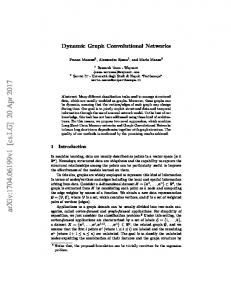
Figure 3. The first images of the first and third rows are the two input image x. Their invariant attribute array x ¯j (vj−1 , vj ) is shown below for j = J − 1, with high amplitude coefficients appearing as white points. Vertical and horizontal axes correspond respectively to vj−1 and vj , so translations of vj−1 by τ are vertical translations. An image xτ in a column τ + 1 has an invariant attribute x ¯τj which is shown below. It is the closest to x ¯j (vj−1 − τ, vj ) in the databasis.

To analyze the effect of this translation, we eliminate variability along vj−2 and define an invariant attribute array by choosing the central spatial position u0 : X x ¯j (vj−1 , vj ) = xj (u0 , vj−2 , vj−1 , vj ). (9) vj−2

We relate this translation to an image in the training dataset by finding the image xτ in the dataset which minimizes k¯ xj (vj−1 − τ, vj ) − x ¯τj (vj−1 , vj )k2 , if this minimum Euclidean distance is sufficiently small. To compute accurately a translation by τ we eliminate the high frequency variations of xj and xτj along vj−1 with a filter which averages consecutive samples, before computing their translation. The network used in this experiment is implemented with circular convolutions to avoid border effects, which have nearly the same classification performance. Figure 3 shows the sequence of xτ obtained with a translation by τ of x ¯j at depth j = J − 1, for two images x in the “bird” class. Since we are close to the ouptut, we expect that translated images belong to the same class. This is not the case for the second image of the first ”Bird 1”. It is a ”car” instead of a ”bird”. This corresponds to a classification error but observe that x ¯τJ−1 is quite different from x ¯J−1 translated. We otherwise observe that in these final layers, translations of x ¯J−1 defines images in the same class. τ

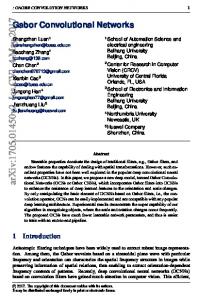
Figure 4 gives sequences of translated attribute images x , computed by translating x ¯j by τ at different depth j and for different input x. As expected, at small depth j, translating an attribute vj−1 does not define images in the same

At deep layers j, translations of x ¯j define images xr which have a progressively higher probability to belong to the same class as x. These attribute transformations correspond to large scale image pattern related to modifications of the filters wvj−1 . In this case, the attribute indices could be interpreted as addresses in organized arrays. The translation group would then correspond to translations of addresses. Understanding better the properties of attributes at different depth is an issue that will be explored in the future.

6. Conclusion Multiscale Hierarchical convolutional networks give a mathematical framework to study invariants computed by deep neural networks. Layers are parameterized in progressively higher dimensional spaces of hierarchical attributes, which are learned from training data. All network operators are multidimensional convolutions along attribute indices, so that invariants can be computed by summations along these attributes. This paper gives image classification results with an efficient implementation computed with a cascade of 5D convolutions and intermediate non-linearities. Invariant are progressively calculated as depth increases. Good classification accuracies are obtained with a reduced number of parameters compared to other CNN. Translations along attributes at shallow depth correspond to low-level image properties at fine scales whereas attributes at deep layers correspond to modifications of large scale pattern structures. Understanding better the multiscale properties of these attributes and their relations to the symmetry group of f is an important issue, which can lead to a better mathematical understanding of CNN learning algorithms.

Acknowledgements This work is funded by STW project ImaGene, ERC grant InvariantClass 320959 and via a grant for PhD Students of the Conseil régional d’Île-de-France (RDMIdF).


x3 x4 x5 x6 x7 x8 x9 x10 x11 Figure 4. The first columns give the input image x, from which we compute the invariant array x ¯j at a depth 3 ≤ j ≤ 11 which increases with the row. The next images in the same row are the images xτ whose invariant arrays x ¯τj are the closest to x ¯j translated by 1 ≤ τ ≤ 7, among all other images in the databasis. The value of τ is the column index minus 1.

References Budden, David, Matveev, Alexander, Santurkar, Shibani, Chaudhuri, Shraman Ray, and Shavit, Nir. Deep tensor convolution on multicores. arXiv preprint arXiv:1611.06565, 2016. Cheng, Yu, Yu, Felix X, Feris, Rogerio S, Kumar, Sanjiv, Choudhary, Alok, and Chang, Shi-Fu. An exploration of parameter redundancy in deep networks with circulant projections. In Proceedings of the IEEE International Conference on Computer Vision, pp. 2857–2865, 2015. Clevert, Djork-Arné, Unterthiner, Thomas, and Hochreiter, Sepp. Fast and accurate deep network learning by exponential linear units (elus). arXiv preprint arXiv:1511.07289, 2015. Denton, Emily L, Zaremba, Wojciech, Bruna, Joan, LeCun, Yann, and Fergus, Rob. Exploiting linear structure within convolutional networks for efficient evaluation. In Advances in Neural Information Processing Systems, pp. 1269–1277, 2014. Goodfellow, Ian J, Vinyals, Oriol, and Saxe, Andrew M.

Qualitatively characterizing neural network optimization problems. arXiv preprint arXiv:1412.6544, 2014. Ha, David, Dai, Andrew, and Le, Quoc V. Hypernetworks. arXiv preprint arXiv:1609.09106, 2016. He, Kaiming, Zhang, Xiangyu, Ren, Shaoqing, and Sun, Jian. Deep residual learning for image recognition. In Proceedings of the IEEE Conference on Computer Vision and Pattern Recognition, pp. 770–778, 2016. Huang, Gao, Liu, Zhuang, Weinberger, Kilian Q, and van der Maaten, Laurens. Densely connected convolutional networks. arXiv preprint arXiv:1608.06993, 2016. Ioffe, Sergey and Szegedy, Christian. Batch normalization: Accelerating deep network training by reducing internal covariate shift. arXiv preprint arXiv:1502.03167, 2015. Jacobsen, Jorn-Henrik, van Gemert, Jan, Lou, Zhongyu, and Smeulders, Arnold WM. Structured receptive fields in cnns. In Proceedings of the IEEE Conference on Computer Vision and Pattern Recognition, pp. 2610–2619, 2016.


Jaderberg, Max, Vedaldi, Andrea, and Zisserman, Andrew. Speeding up convolutional neural networks with low rank expansions. arXiv preprint arXiv:1405.3866, 2014. Krizhevsky, Alex and Hinton, G. Convolutional deep belief networks on cifar-10. Unpublished manuscript, 40, 2010. Krizhevsky, Alex, Sutskever, Ilya, and Hinton, Geoffrey E. Imagenet classification with deep convolutional neural networks. In Advances in neural information processing systems, pp. 1097–1105, 2012. LeCun, Yann, Boser, Bernhard, Denker, John S, Henderson, Donnie, Howard, Richard E, Hubbard, Wayne, and Jackel, Lawrence D. Backpropagation applied to handwritten zip code recognition. Neural computation, 1(4): 541–551, 1989. LeCun, Yann, Kavukcuoglu, Koray, and Farabet, Clément. Convolutional networks and applications in vision. In Circuits and Systems (ISCAS), Proceedings of 2010 IEEE International Symposium on, pp. 253–256. IEEE, 2010. LeCun, Yann, Bengio, Yoshua, and Hinton, Geoffrey. Deep learning. Nature, 521(7553):436–444, 2015. Lu, Zhiyun, Sindhwani, Vikas, and Sainath, Tara N. Learning compact recurrent neural networks. In Acoustics, Speech and Signal Processing (ICASSP), 2016 IEEE International Conference on, pp. 5960–5964. IEEE, 2016. Mallat, Stéphane. Understanding deep convolutional networks. Phil. Trans. R. Soc. A, 374(2065):20150203, 2016. Oyallon, Edouard and Mallat, Stéphane. Deep rototranslation scattering for object classification. In Proceedings of the IEEE Conference on Computer Vision and Pattern Recognition, pp. 2865–2873, 2015. Romero, Adriana, Ballas, Nicolas, Kahou, Samira Ebrahimi, Chassang, Antoine, Gatta, Carlo, and Bengio, Yoshua. Fitnets: Hints for thin deep nets. arXiv preprint arXiv:1412.6550, 2014. Springenberg, Jost Tobias, Dosovitskiy, Alexey, Brox, Thomas, and Riedmiller, Martin. Striving for simplicity: The all convolutional net. arXiv preprint arXiv:1412.6806, 2014. Zagoruyko, Sergey and Komodakis, Nikos. Paying more attention to attention: Improving the performance of convolutional neural networks via attention transfer. arXiv preprint arXiv:1612.03928, 2016. Zeiler, Matthew D and Fergus, Rob. Visualizing and understanding convolutional networks. In European conference on computer vision, pp. 818–833. Springer, 2014.