Introduction. This issue paper explains when and how to apply first-order attenuation rate constant calculations in monitored natural attenuation (MNA) studies.
United States Environmental Protection Agency
Ground Water Issue
Calculation and Use of First-Order Rate Constants for Monitored Natural Attenuation Studies Charles J. Newell1, Hanadi S. Rifai2, John T. Wilson3, John A. Connor1, Julia A. Aziz1, and Monica P. Suarez2
Introduction
or concentration of contaminants in soil and ground water. These in-situ processes include biodegradation, dispersion, dilution, sorption, volatilization; radioactive decay; and chemical or biological stabilization, transformation, or destruction of contaminants (U.S. EPA, 1999).
This issue paper explains when and how to apply first-order attenuation rate constant calculations in monitored natural attenuation (MNA) studies. First-order attenuation rate constant calculations can be an important tool for evaluating natural attenuation processes at ground-water contamination sites. Specific applications identified in U.S. EPA guidelines (U.S. EPA, 1999) include use in characterization of plume trends (shrinking, expanding, or showing relatively little change), as well as estimation of the time required for achieving remediation goals. However, the use of the attenuation rate data for these purposes is complicated as different types of first-order rate constants represent very different attenuation processes:
The overall impact of natural attenuation processes at a given site can be assessed by evaluating the rate at which contaminant concentrations are decreasing either spatially or temporally. Recent guidelines issued by the U.S. EPA (U.S. EPA, 1999) and the American Society for Testing and Materials (ASTM, 1998) have endorsed the use of site-specific attenuation rate constants for evaluating natural attenuation processes in ground water. The U.S. EPA directive on the use of Monitored Natural Attenuation (MNA) at Superfund, RCRA, and UST sites (U.S. EPA, 1999) includes several references to the application of attenuation rates:
Concentration vs. time rate constants ( kpoint ) are used for estimating how quickly remediation goals will be met at a site.
Once site characterization data have been collected and a conceptual model developed, the next step is to evaluate the potential efficacy of MNA as a remedial alternative. This involves collection of site-specific data sufficient to estimate with an acceptable level of confidence both the rate of attenuation processes and the anticipated time required to achieve remediation objectives.
Concentration vs. distance bulk attenuation rate constants ( k ) are used for estimating if a plume is expanding, showing relatively little change, or shrinking due to the combined effects of dispersion, biodegradation, and other attenuation processes. Biodegradation rate constants ( λ ) are used in solute transport models to characterize the effect of biodegradation on contaminant migration.
At a minimum, the monitoring program should be sufficient to enable a determination of the rate(s) of attenuation and how that rate is changing with time.
Correct use of attenuation rate constants requires an understanding of the different attenuation processes that different first-order rate constants represent.
Site characterization (and monitoring) data are typically used for estimating attenuation rates.
For further information contact John T. Wilson (580) 436-8534 at the Subsurface Protection and Remediation Division of the National Risk Management Research Laboratory, Office of Research and Development, U.S. Environmental Protection Agency, Ada, Oklahoma.
The ASTM Standard Guide for Remediation of Groundwater by Natural Attenuation at Petroleum Release Sites (ASTM, 1998) also identifies site-specific attenuation rates as a secondary line of evidence of the occurrence and rate of natural attenuation. In addition, technical guidelines issued by various state environmental regulatory agencies recommend estimation of rate constants to evaluate contaminant plume trends and duration (New Jersey DEP, 1998; Wisconsin DNR, 1999). For example, the New Jersey Department of Environmental Protection (DEP) now requires such calculations for establishing “Classification Exception Areas (CEAs)” at sites where ground-water quality standards are or will be exceeded for an extended time period.
Why Are Attenuation Rate Constants Important? Monitored natural attenuation (MNA) refers to the reliance on natural attenuation processes to achieve site-specific remediation objectives within a reasonable time frame. Natural attenuation processes include a variety of physical, chemical, and/or biological processes that act without human intervention to reduce the mass 1
Groundwater Services, Inc., Houston, Texas
2
University of Houston, Texas
The technical literature contains numerous guidelines regarding methods for derivation of site-specific attenuation rate constants based upon observed plume concentration trends (e.g., ASTM, 1998; U.S. EPA, 1998a; 1998b; Wiedemeier et al. 1995; 1999; Wilson and Kolhatkar, 2002). Other resources, such as the
3 U.S. Environmental Protection Agency, Office of Research and Development, National Risk Management Research Laboratory, Subsurface Protection and Remediation Division, Ada, Oklahoma
1
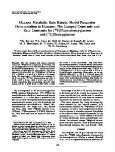
contaminant transport vs. transport of a tracer, or more commonly, calibration of solute transport model to field data (Figure 3).
BIOSCREEN and BIOCHLOR natural attenuation models (Newell et al., 1996; Aziz et al., 2000), include use of first-order rate constants for simulating the attenuation of dissolved contaminants once they leave the source and the attenuation of the source itself. However, many of these references do not clearly distinguish between the different types of rate constants and their appropriate application in evaluation of natural attenuation processes. The objective of this paper is to address this gap by briefly describing the derivation, significance, and appropriate use of three key types of attenuation rate constants commonly employed in natural attenuation studies.
Contam . λ Tracer
λ=0
Key Point:
Find λ
Rate calculations can help those performing MNA studies evaluate the contribution of attenuation processes and the anticipated time required to achieve remediation objectives. There are different types of rate calculations, however, and it is important to use the right kind of rate constant for the right application.
Figure 3.
Distinctions Between Rate Constants To interpret the past behavior of plumes, and to forecast their future behavior, it is necessary to describe the behavior of the plume in both space and time. It is necessary to collect long-term monitoring data from wells that are distributed throughout the plume. Concentration vs. Time Rate Constants describe the behavior of the plume at one point in space; while Concentration vs. Distance Rate Constants describe the behavior of the entire plume at one point in time. The Biodegradation Rate Constant is usually applied over both time and space, but only applies to one attenuation mechanism. Standard practice for the environmental industry finds applications for each of these rate constants. Under appropriate conditions, each of the three constants can be employed to assist in site-specific evaluation and quantification of natural attenuation processes. Each of these terms is identified as an “attenuation rate.” Because they differ in their significance and appropriate application, it is important to understand the potential for misapplication of each type of rate as summarized below:
Types of First-Order Attenuation Rate Constants In general, there are three different types of first-order attenuation rate constants that are in common use:
Nat. Log Concentration
Concentration vs. Time Attenuation Rate Constant, where a rate constant, in units of inverse time (e.g., per day), is derived as the slope of the natural log concentration vs. time curve measured at a selected monitoring location (Figure 1).
k point = Slope
Time
Figure 1.
Concentration vs. Time Rate Constants: A rate constant derived from a concentration vs. time (C vs. T) plot at a single monitoring location provides information regarding the potential plume lifetime at that location, but cannot be used to evaluate the distribution of contaminant mass within the ground-water system. The C vs. T rate constant at a location within the source zone represents the persistence in source strength over time and can be used to estimate the time required to reach a remediation goal at that particular location. To adequately assess an entire plume, monitoring wells must be available that adequately delineate the entire plume, and an adequate record of monitoring data must be available to calculate a C vs. T plot for each well. At most sites, the rate of attenuation in the source area (due to weathering of residual source materials such as NAPLs) is slower than the rate of attenuation of materials in ground water, and concentration profiles in plumes tend to retreat back toward the source over time. In this circumstance, the lifecycle of the plume is controlled by the rate of attenuation of the source, and can be predicted by the C vs. T plots in the most contaminated wells. At some sites, the rate of attenuation of the source is rapid compared to the rate of attenuation in ground water. This pattern is most common when contaminants are readily soluble in ground water and when contaminants are not biodegraded in ground water. In this case, the rate of attenuation of the source as predicted by a C vs. T plot will underestimate the lifetime of the plume.
Determining concentration vs. time rate constant (kpoint).
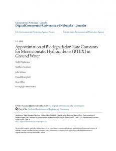
Concentration vs. Distance Attenuation Rate Constant, where a rate constant, in units of inverse time (e.g., per day), is derived by plotting the natural log of the concentration vs. distance and (if determined to match a first-order pattern) calculating the rate as the product of the slope of the transformed data plot and the ground-water seepage velocity (Figure 2).
Nat. Log Concentration
Determining biodegradation rate constant ( λ ).
SLOPE = k/ Vgw
Distance from Source
Figure 2. Determining concentration vs. distance rate constant (k). Biodegradation Rate Constant. The “biodegradation rate constant” ( λ ) in units of inverse time (e.g., per day) can be derived by a variety of methods, such as comparison of
Concentration vs. Distance Rate Constants: Attenuation rate constants derived from concentration vs. distance (C vs. D)
2
plots serve to characterize the distribution of contaminant mass within space at a given point in time. A single C vs. D plot provides no information with regard to the variation of dissolved contaminant mass over time and, therefore, cannot be employed to estimate the time required for the dissolved plume concentrations to be reduced to a specified remediation goal. This rate constant incorporates all attenuation parameters (sorption, dispersion, biodegradation) for dissolved constituents after they leave the source. Use of the rate constant derived from a C vs. D plot (i.e., characterization of contaminant mass over space) for this purpose (i.e., to characterize contaminant mass over time) will provide erroneous results. The C vs. D-based rate constant indicates how quickly dissolved contaminants are attenuated once they leave the source but provides no information on how quickly a residual source zone is being attenuated. Note that most sites with organic contamination will have some type of continuing residual source zone, even after active remediation (Wiedemeier et al., 1999), making the C vs. D rate constant inappropriate for estimating plume lifetimes for most sites.
describe the first-order decay process, while others prefer half-lives. These two terms are linearly related by: Rate constant = 0.693 / [ half-life ] and Half-life = 0.693 / [ rate constant ] For example, a 2 year half-life is equivalent to a first-order rate constant of 0.35 per year. This document describes the firstorder decay process in terms of rate constants instead of halflives.
Key Point: Rate constants and half-lives represent the same first-order decay process, and are inversely related.
Appropriate Use of Attenuation Rate Constants in Natural Attenuation Studies Attenuation rate constants may be used for the following three purposes in natural attenuation studies: Plume Attenuation: Demonstrate that contaminants are being attenuated within the ground-water flow system;
Biodegradation Rate Constant: Another type of error occurs if a C vs. D rate constant is used as the biodegradation rate term ( λ ) in a solute transport model. The attenuation rate constant derived from the C vs. D plot already reflects the combined effects of contaminant sorption, dispersion, and biodegradation. Consequently, use of a C vs. D rate constant as the biodegradation rate within a model that separately accounts for sorption and dispersion effects will significantly overestimate attenuation effects during ground-water flow.
Plume Trends: Determine if the affected ground-water plume is expanding, showing relatively little change, or shrinking; and Plume Duration: Estimate the time required to reach groundwater remediation goals by natural attenuation alone. Appropriate use of the various attenuation rate constants for evaluation of plume attenuation, trends, and duration is shown in Table 1.
These examples serve to illustrate the need to ensure an appropriate match between the significance and use of each rate constant. Further guidelines regarding derivation and use of attenuation rate constants are provided below.
As described in the U.S. EPA MNA Directive (U.S. EPA, 1999): Site characterization (and monitoring) data are typically used for estimating attenuation rates. These calculated rates may be expressed with respect to either time or distance from the source. Time-based estimates are used to predict the time required for MNA to achieve remediation objectives and distance-based estimates provide an evaluation of whether a plume will expand, remain stable, or shrink.
Key Point: There are three general types of first-order rate constants that are commonly used for MNA studies: (1) Concentration vs. Time, (2) Concentration vs. Distance, and (3) Biodegradation.
Rate Constants vs. Half-Lives
To clarify the applicability of the various first-order decay rate constants, appropriate nomenclature is useful to indicate the significance of each term. For example, point decay rates (defined
Both first-order rate constants and attenuation half-lives represent the same process, first-order decay. Some environmental professionals prefer to use rate constants (in units of per time) to Table 1.
Summary of First-Order Rate Constants for Natural Attenuation Studies
Rate Constant Point Attenuation Rate (Fig. 1) (kpoint, time per year) Bulk Attenuation Rate (Fig. 2) (k; time per year) Biodegradation Rate (Fig. 3) (λ, time per year)
Method of Analysis
C vs. T Plot
C vs. D Plot
Model Calibration, Tracer Studies, Calculations
Significance Reduction in contaminant concentration over time at a single point Reduction in dissolved contaminant concentration with distance from source Biodegradation rate for dissolved contaminants after leaving source, exclusive of advection, dispersion, etc.
Use of Rate Constant Plume Plume Plume Attenuation Trends? Duration? NO*
NO*
YES
YES
NO*
NO
YES
NO
NO
* Note: Although assessment of an attenuation rate constant at a single location does not yield plume attenuation information, or plume trend information, an assessment of general trends of multiple wells over the entire plume is useful to assess overall plume attenuation and plume trends.
3
as kpoint) , derived from single well concentration vs. time plot, may be used to determine how long a plume will persist (Plume Duration). While concentration vs. time data at a single point in the plume are useful for determining trends at that location (i.e., are concentrations increasing, showing relatively little change, or declining), a rate constant calculated from concentration vs. time data at a single location cannot be used to estimate the trend of an entire plume.
in flow direction. See Hyman and DuPont, 2001 and DuPont et al.,1998 for discussion and details of the methods. Mass Flux vs. Distance Rate Constant. A mass vs. distance decay rate (in units of inverse time) can be calculated by plotting the natural log of mass flux through different transects perpendicular to the flow as a function of distance from the source and multiplying the slope of the best-fit line by the seepage velocity. Comparable to the bulk attenuation rate, this type of rate can be used to indicate if a plume is expanding, showing relatively little change, or shrinking. See Einarson and Mackay, 2001 for examples of mass flux calculations. Another method for calculating mass loss rates is described by the Remediation Technologies Development Forum (RTDF, 1997).
Bulk attenuation rates (defined as k), derived from concentration vs. distance plots, can be used to indicate if a plume is expanding, showing relatively little change, or shrinking (Plume Trends). Biodegradation rates ( λ ), modeling parameters which are specific to biodegradation effects and exclusive of dispersion, etc., can be used in appropriate solute transport models to indicate if a plume is expanding, showing relatively little change, or shrinking (Plume Trends).
Mass Flux-Based Biodegradation Rate Constant. Mass fluxes across plume transects can be further analyzed to determine whether the observed mass loss spatially and temporally can be attributed to biodegradation and/or source decay. For this purpose, the mass flux across the source area is compared to the mass flux through the next downgradient section. Theoretically, mass fluxes at the downgradient transect should mimic the trends observed in the source transect if source decay, sorption, and dispersion were the only mass reduction attenuation mechanisms. If there is additional mass loss, it can only be attributed to biodegradation since the other processes are already accounted for in the mass flux calculation. Once the actual mass loss attributable to biodegradation has been determined, it is plotted as a function of time and a biodegradation rate is estimated using linear regression or a first-order decay model fit to the data. See Borden et al. (1997) and Semprini et al. (1995) for examples of biodegradation rates calculated from mass flux across transects.
For each of these first-order decay rate parameters, Table 2 summarizes information on the derivation and appropriate use as well as providing representative values. In summary, different types of first-order attenuation rate calculations are available to help evaluate natural attenuation processes at contaminated ground-water sites. These different types of rate constants represent different types of attenuation processes, therefore, the right type of rate constant should be used for the right purpose. Examples 1-3 illustrate how the three types of rate constants are calculated and applied.
Key Point: In general, all three types of rate constants are useful indicators that attenuation is occurring. Concentration vs. time rate constants ( kpoint ) can be used to estimate the duration of contamination at a particular location. Concentration vs. time rate constants for wells encompassing the entire plume can be used to identify overall trends and predict the duration of the plume. Concentration vs. distance rate constants ( k ) and biodegradation rate constants ( λ ) can be used to project the rate of attenuation of contaminants along the flow path in ground water, and predict the spatial extent of the plume.
Mass-based rate constants are not often used in practice due to the data needs for mass estimates including a dense well network as well as localized gradients, conductivity measurements, and aquifer thickness at monitoring points. Average-Plume Concentration Rate Constants. Some researchers and practitioners have calculated rate constants for the change in average plume concentration. This rate constant reflects primarily the change in source strength over time.
Effect of Residual NAPL on Point Decay Rate Constant
Tables 1 and 2 provide more detail on use, calculations, and analysis of the three types of rate constants. Examples 1-3 illustrate the use and application of the three types of rate constants.
When a monitoring well is screened across an interval that contains residual NAPL, and when the rate of weathering of the NAPL is slow, the well water may sustain high concentrations of contaminants over long periods of time.
Other Types of Rate Constants Mass-Based Rate Constants. The previous discussion focused on concentration-based rates. It is also possible to calculate mass vs. time rate constants and mass vs. distance rate constants. In practice, these rates would be very similar to the concentrationbased rates.
Effect of NA Processes on Rate Constants Natural attenuation processes include a variety of physical, chemical, or biological processes that act without human intervention to reduce the mass or concentration of contaminants in soil and ground water. These in-situ processes include biodegradation, dispersion, dilution, sorption, volatilization, radioactive decay, and chemical or biological stabilization, transformation, or destruction of contaminants (U.S. EPA, 1999).
Mass vs.Time Rate Constant. This constant compares changes in the total mass of contaminants in the plume over time. A Thiessen polygon network can be used to weight the concentration data from all the available wells at a site to derive a comprehensive estimate of the mass of contaminants in the plume at any particular round of sampling. Mass vs. time decay rates (in units of inverse time) are estimated by plotting the natural log of total dissolved mass as a function of time and estimating the slope of the line. This rate is similar to the concentration vs. time rate and since it accounts for the entire plume, it is a good indicator of how long a plume will persist. Many plumes change flow direction over time, making it difficult to identify a stable centerline. Estimates based on the entire plume are less subject to errors caused by changes
Each of these processes influences contaminant concentrations in soil and ground water both spatially and temporally at a site. Contaminant concentrations in ground water are reduced as they travel downgradient from the source. Subject to source degradation, contaminant concentrations will also be reduced with time at any given distance downgradient from the source. These concepts are illustrated in Appendices II and III. The data in Appendix II illustrate the change in contaminant concentrations downgradient from the source at a hypothetical site in response
4
to the different attenuation processes. It can be clearly seen from Appendix II that contaminant concentrations downgradient from source areas are attenuated due to dispersion, sorption, biodegradation and source decay.The data in Appendix III illustrate the change in contaminant concentrations with time at two points downgradient from the source at the hypothetical site (one point near the source and the other point at the leading edge of the plume). As can be seen from Appendix III, contaminant concentrations near the source will attenuate with time only if source decay is occurring. While source decay is also important for the leading edge of the plume, maximum contaminant concentrations in that zone are significantly attenuated from their source concentration counterparts due to biodegradation, sorption, and dispersion.
Uncertainty in Rate Calculations Rate calculations can be affected by uncertainty from a number of sources, such as the design of the monitoring network, seasonal variations, uncertainty in sampling methods and lab analyses, and the heterogeneity in most ground-water plumes. Appendix I discusses uncertainty in rate calculations and provides methods for managing this uncertainty. ORD has developed software (RaCES) to extract rate constants from field data. This software is intended to facilitate an evaluation of the uncertainty associated with the projections made by computer models of the future behavior of plumes of contamination in ground water. The software is available from The Ecosystem Research Division of the National Exposure Research Laboratory in Athens, Georgia (Budge et al., 2003).
Notice The U.S. Environmental Protection Agency through its Office of Research and Development funded and managed the research described here under Contract No. 68-C-99-256 to Dynamac Corporation. It has been subjected to the Agency’s peer and administrative review and has been approved for publication as an EPA document. Mention of trade names or commercial products does not constitute endorsement or recommendation for use.
Quality Assurance Statement All research projects making conclusions or recommendations based on environmental data and funded by the U.S. Environmental Protection Agency are required to participate in the Agency Quality Assurance Program. This project did not involve the collection or use of environmental data and, as such, did not require a Quality Assurance Project Plan.
5
Table 2.
Quick Reference Summary of Three Types of Attenuation Rate Constants Point Decay Rate Constant (k point)
Bulk Attenuation Rate Constant (k )
Biodegradation Rate Constant ( λ )
USED FOR:
Plume Duration Estimate. Used to estimate time required to meet a remediation goal at a particular point within the plume. If wells in the source zone are used to derive k point, then this rate can be used to estimate the time required to meet remediation goals for the entire site. k point should not be used for representing biodegradation of dissolved constituents in ground-water models (use λ as described in the right hand column).
Plume Trend Evaluation. Can be used to project how far along a flow path a plume will expand. This information can be used to select the sites for monitoring wells and plan long-term monitoring strategies. Note that k should not be used to estimate how long the plume will persist except in the unusual case where the source has been completely removed, as the source will keep replenishing dissolved contaminants in the plume.
Plume Trend Evaluation. Can be used to indicate if a plume is still expanding, or if the plume has reached a dynamic steady state. First calculate λ, then enter λ into a fate and transport model and run the model to match existing data. Then increase the simulation time in the model and see if the plume grows larger than the plume simulated in the previous step. Note that λ should not be used to estimate how long the plume will persist except in the unusual case where the source has been completely removed.
REPRESENTS:
Mostly the change in source strength over time with contributions from other attenuation processes such as dispersion and biodegradation. k point is not a biodegradation rate as it represents how quickly the source is depleting. In the rare case where the source has been completely removed (for a discussion of source zones, see Wiedemeier et al., 1999), k point will approximate k . Plot natural log of concentration vs. time for a single monitoring point and calculate k point = slope of the best-fit line (ASTM, 1998). This calculation can be repeated for multiple sampling points and for average plume concentration to indicate spatial trends in k point as well.
Attenuation of dissolved constituents due The biodegradation rate of dissolved constituents once they have left the to all attenuation processes (primarily sorption, dispersion, and biodegradation). source. It does not account for attenuation due to dispersion or sorption.
k point = Slope
Time
Note this calculation does not account for any changes in attenuation processes, particularly Dual-Equilibrium Desorption (availability) which can reduce the apparent attenuation rate at lower concentrations (e.g., see Kan et al., 1998).
Plot natural log of conc. vs. distance. If the data appear to be first-order, determine the slope of the natural logtransformed data by: 1. Transforming the data by taking natural logs and performing a linear regression on the transformed data, or
Adjust contaminant concentration by comparison to existing tracer (e.g., chloride, tri-methyl benzenes) and then use method for bulk attenuation rate (see Wiedemeier et al., 1999); or Calibrate a ground-water solute transport computer model that includes dispersion and retardation (e.g., BIOSCREEN, BIOCHLOR, BIOPLUME III, MT3D) by adjusting λ; or
2. Plotting the data on a semi-log plot, taking the natural log of the y intercept minus the natural log of the x intercept and dividing by the distance between the Use the method of Buscheck and two points. Alcantar (1995) (plume must be at steady-state to apply this method). Note Multiply this slope by the contaminant this method is a hybrid between k and λ velocity (seepage velocity divided by the as the Buscheck and Alcantar method retardation factor R) to get k . removes the effects of longitudinal dispersion, but does not remove the effects of transverse dispersion from their λ.
Contam . λ Tracer
Nat. Log Concentration
Nat. Log Concentration
HOW TO CALCULATE:
SLOPE = k/ Vgw
λ=0 Find λ
Distance from Source
6
Table 2.
Continued... Point Decay Rate Constant (k point)
HOW TO USE:
Bulk Attenuation Rate Constant (k)
To estimate plume lifetime:
To estimate if a plume is showing relatively little change:
The time (t) to reach the remediation goal at the point where K point was calculated is:
Pick a point in the plume but downgradient of any source zones. Estimate the time needed to decay these dissolved contaminants to meet a remediation goal as these contaminants move downgradient:
C −Ln goal Cstart t= k point
C −Ln goal Cstart t= k
Biodegradation Rate Constant ( λ ) To estimate if a plume is showing relatively little change: Enter λ in a solute transport model that is calibrated to existing plume conditions. Increase the simulation time (e.g. by 100 years, or perhaps to the year 2525), and determine if the model shows that the plume is expanding, showing relatively little change, or shrinking.
Calculate the distance L that the dissolved constituents will travel as they are decaying using Vs as the seepage velocity and R is the retardation factor for the contaminant:
L=
Vs ⋅t R
If the plume currently has not traveled this distance L then this rate analysis suggests the plume may expand to that point. If the plume has extended beyond point L, then this rate analysis suggests the plume may shrink in the future. Note that an alternative (and probably easier method) is to merely extrapolate the regression line to determine the distance where the regression line reaches the remediation goal. TYPICAL VALUES:
Reid and Reisinger (1999) indicated that the mean point decay rate constant for benzene from 49 gas station sites was 0.46 per year (half-life of 1.5 years). For MTBE they reported point decay rate constants of 0.44 per year (half-life of 1.6 years). In contrast, Peargin (2002) calculated rates from wells that were screened in areas with residual NAPL; the mean decay rate for MTBE was 0.04 per year (half life of 17 years) the rate for benzene was 0.14 per year (half life of 5 years).
For many BTEX plumes, k will be similar to biodegradation rates λ (on the order of 0.001 to 0.01 per day; see Figure 4) as the effects of dispersion and sorption will be small compared to biodegradation.
For BTEX compounds, 0.1 - 1 %/day (half-lives of 700 to 70 days)(Suarez and Rifai, 1999). Chlorinated solvent biodegradation rates may be lower than BTEX biodegradation rates at some sites (Figures 4 and 5).
For more information about biodegradation rates for a variety of compounds, see Wiedemeier et al., 1999 and Suarez and Rifai, 1999.
Newell (personal communication) calculated the following median point decay rate constants: 0.33 per year (2.1 year half-life) for 159 benzene plumes at service station sites in Texas; and 0.15 per year (4.7 year half-life) for 37 TCE plumes around the U.S.
7
10
LEGEND
0.07
0.7
25 Percentile
Minimum
7 Benzene
0.01
70
Typical Decay Rate Range: 0.1% to 1% per day
700
0.001
25 percent.: 0 Min: 0
25 percent.: 0 Min: 0
0.0001
Type Rate Const: Source: Number: Field or Lab: Constituents:
λ
λ
7,000
λ
k and λ
Suarez & Rifai, 1999
Suarez & Rifai, 1999
Wied. et al, 1999
Rifai & Newell, 2002
35-50 studies
23-61 studies
23 Air Force sites
66 Florida Gas Stations
Field Only
Lab Only
Field Only
Field
B, T, E, X
Benzene
BTEX
Benzene and BTEX
Rifai et al, 1995 14 sites Field Only Benzene
Biodegradation Rate Constants ( λ ) and Bulk Attenuation Rate Constants (k) for BTEX compounds from the literature. Source: Rifai and Newell, 2001.
LEGEND Maximum 75 Percentile Median 25 Percentile Minimum
Biodegradation Rate Constant λ (per day)
0.1
7 days
0.01
70 days (~0.2 yrs)
0.001
700 days (~1.9 yrs)
0.0001
7000 days (~19yrs)
Constituent Number of Sites
TCE TCE 10
cDCE cDCE 9
Approximate Half-Life
Figure 4.
λ
APPROXIMATE HALF LIFE (DAYS)
Median
Benzene, BTEX
Benzene Anaerobic
Benzene Aerobic
m-Xylene
BTEX
0.1
75 Percentile
Benzene
RATE CONSTANT (Per Day)
1
EthylBenzene
Toluene
Maximum
VC VC 7
Figure 5. Biodegradation Rate Constants ( λ ) for Trichloroethene (TCE), cis-Dichloroethene (cDCE), and Vinyl Chloride (VC) compounds from BIOCHLOR modeling studies. Source: Aziz et al., 2000.
8
EXAMPLE 1. Use of Concentration vs. Time Rate Constants (kpoint ) INTRODUCTION: A leaking underground storage tank site in Elbert, Anystate, has a maximum source concentration of 1.800 mg/L of benzene at well MW-3. A remediation goal of 0.005 mg/L of benzene has been established. How long will it take for this site to reach the remediation goal using MNA with no active remediation? (Data source: Mace et al. 1997) 10
DATA:
KEY POINT: The kpoint degradation rate constant is +0.77 per year. QUESTION: Why is the sign positive? ANSWER: The rate constant is defined as a rate of degradation. The slope of the line is the rate of change. If the slope is negative, then concentrations are attenuating, and the rate of degradation is positive.
DATE 8/19/86 7/17/87 9/29/87 12/19/87 6/25/88 9/30/88 12/21/88 4/25/89 10/23/89 7/4/91 11/20/91
Years Since 1/1/86 0.63 1.54 1.74 1.96 2.48 2.75 2.97 3.31 3.81 5.50 5.88
MW-3 Benzene (mg/L) 1.800 0.440 0.370 0.320 0.270 0.260 0.260 0.220 0.110 0.030 0.018
Benzene Concentration (mg/L)
The following are data from well MW-3 for the period 1986 to 1991. 1
Calculation Tip: If you calculate the slope of the line with a calculator or with a spreadsheet, you need to change the sign to get a degradation rate constant.
0.1
y = 1.9568e-0.7676x 0.01
Benzene MCL (0.005 mg/L) 0.001 0
1
2
4
3
5
6
7
8
9
Time (years since 1/1/86)
CALCULATION: Construct a plot of concentration vs. time. Although the plot can be developed in many ways, the clearest way is to convert the time data to years using an arbitrary starting point (for this example we chose 1/1/86). By transforming the concentrations to natural log concentration, and using a spreadsheet or calculator to get the slope (-0.77) and intercept (0.67), the following equation of the line was generated: Ln ( Conc. Benzene) = exp (0.67-0.77x)
which resulted in the following rate equation:
Benzene concentration (mg/L) = 1.96 mg/L* exp (- 0.77 yrs since 1/1/86)
where kpoint = +0.77 per year.
Rearranging the equation: Time (years since 1/1/86) = - Ln [ Conc. Benzene (mg/L) / 1.96 ] / 0.77 For the case where the remediation goal is 0.005 mg/L benzene, Time (years since 1/1/86) = - Ln [ 0.005 / 1.96 ] / 0.77 = 7.7 years = late 1993 A statistical analysis of the uncertainty involved in the calculation can be performed by determining the “one tailed” 90% confidence interval using the methods outlined in Appendix I. The “one tailed” 90% confidence limit on the time to remediation is a time that is no longer than 8.6 years from 1/1/86, or late 1994. Plume Attenuation? The concentration vs. time rate constant is positive, indicating that attenuation at this location (the source zone in this example) is occurring. The attenuation is probably due to weathering of the source caused by dissolution of benzene from a residual NAPL into flowing ground water. Raoult’s Law predicts that weathering from dissolution will be a first-order process.
Plume Trends? The concentration vs. time rate constant is positive, indicating that concentrations in this portion of the plume are going down and that at least a portion of the plume may be shrinking. However, from the information obtained at a single location, no conclusion can be drawn regarding the overall plume trend.
Plume Duration? The concentration vs. time rate constant was used to show that if current trends hold then the plume will reach the clean-up goal in 1994. Note this assessment does not consider any other processes which could reduce the observed attenuation rate (i.e., changes in water levels, availability effects at low concentration as described by Kan et al., 1998, etc.).
Key Point: A concentration vs. time rate constant is one of the best ways to estimate how long MNA (or any type of remediation system) might take to reach a clean-up goal. A second method is to perform a mass-based approach (i.e., see DuPont et al., 1998; Hyman and DuPont, 2001; Newell et al., 1996 or Chapter 2 of Wiedemeier et al., 1999).
9
EXAMPLE 2. Use of Concentration vs. Distance Rate Constants (k) INTRODUCTION: This constant is estimated between wells along the inferred centerline of the plume. An MTBE plume at a former fuel farm located at a U.S. Coast Guard Base has a maximum source zone concentration of 1.740 mg/L of MTBE. The average calculated seepage velocity at the site was calculated to be 82 meters per year and the retardation factor, R, is assumed to be equal to one. For the purpose of this example, a clean-up goal of 0.030 mg/L was assumed. Most importantly, the site is strongly anaerobic, indicating that relatively high rates of MTBE biodegradation are possible. Is the MTBE plume 10 attenuating? How far should it extend? (source: Wilson et al., 2000). DATA: The following is data from wells along the plume centerline: Well
Distance from
Source(m) CPT-1 0 CPT-3 40 CPT-5 70 ESM-14 104 ESM-3 134 ESM-9 180 ESM-10 195 GP-1 250
MTBE Conc.(mg/L) 1.74 0.823 0.672 0.383 0.319 0.001 0.0097 0.001
MTBE Concentration (mg/L)
Key Point: The degradation rate constant k is + 0.0033 per year. 1
0.1
y = 4.3561e-0.0333x R2 = 0.828
0.01
0.001 0
50
100
150
200
250
300
Distance from Source (meters)
CALCULATION: First, plot the natural log of concentration vs. distance at a point in time and calculate the slope of the best-fit line using linear regression analysis, as shown above. The slope of the C vs. D plot is -0.033 per meter of travel. Next, calculate the bulk attenuation rate constant, k, by multiplying the negative of the slope of the regression by the contaminant velocity. The contaminant velocity equals the seepage velocity divided by the retardation factor. In this case the retardation factor is 1, and the contaminant velocity is 82 meters per year. The bulk attenuation rate is (+0.033 per meter) * (82 meter per year) = 2.7 per yr. This corresponds to a dissolved-phase half-life of 0.26 yrs (0.26 yrs = 0.69 / 2.7 per yr) after the MTBE leaves the source zone. To estimate the travel time required for the concentration of MTBE to attenuate to the cleanup goal, use the equation in Table 2. The travel time to reach the remediation goal at the down gradient margin of the plume is 1.5 years (1.5 yr = - Ln [0.030 mg/L/ 1.74 mg/L] / 2.7 per y). Based on the calculated attenuation rate, an MTBE source concentration of 1.74 mg/L, and a cleanup goal of 0.030 mg/L, the MTBE plume should extend 123 meters from the source (123 meters = 82 meters per yr * 1.5 yr travel time). A sensitivity analysis can be performed on the rate estimates. See Appendix I for a discussion of confidence intervals. The one-tailed 95% confidence interval on the slope is -0.021 per foot. At a seepage velocity of 82 meters per year, this is equivalent to a concentration vs. distance rate constant (k) of 1.7 per year. The plume would require 2.4 years of travel in the aquifer to attenuate to the cleanup goal. At 95% confidence, the plume boundary would be no more than 200 meters from the source. The estimate of seepage velocity is also subject to uncertainty. A reasonable upper boundary on the seepage velocity at this site is 150 meters per year (Wilson et al., 2000). At the upper bound on seepage velocity, and at the 95% confidence interval on the slope, the MTBE plume would extend no more than 360 meters. Plume Attenuation? The calculated concentration vs. distance rate constant is positive, indicating that attenuation of dissolved MTBE is occurring after the MTBE leaves the source zone. The rate constant of 2.7 per year indicates that dissolved MTBE concentrations will be reduced by 50% every 0.25 yrs after the MTBE leaves the source zone. It does not indicate the entire plume will be reduced in concentration by 50% in 0.25 yrs.
Plume Trends? In theor y, the concentration vs. distance rate constant can provide supporting evidence that the plume may be showing relatively little change or shrinking in the future. However, an analysis of concentration vs. time data for all locations within an adequately delineated plume is a much more direct and robust method for estimating plume trends.
Plume Duration? A concentration vs. distance rate constant is not useful for estimating plume duration (i.e., the time to reach a clean-up goal). A mass-based analysis by Wilson et al., 2000 indicated that 60 years might be required to reach the clean-up goal.
Key Point: Concentration vs. distance rate constants cannot be used for estimating remediation time frames, and are only marginally useful for estimating plume trends. This type of rate constant is most useful to predict the boundaries of a plume. It can be used to plan the location of monitoring wells or sentinel wells. This rate constant is also used with other information to calculate the rate of biodegradation.
10
λ). Example 3. Use of Biodegradation Rate Constants (λ IINTRODUCTION: A chlorinated solvent plume at the Cape Canaveral Air Force Base, Florida, has maximum source concentrations of 0.056 mg/L Tetrachloroethene (PCE), 15.8 mg/L Trichloroethene (TCE), 98.5 mg/L cis-Dichloroethene (DCE), and 3.08 mg/L Vinyl Chloride (VC), 33 years after the spill originally occurred. The calculated seepage velocity at the site is 111.7 ft per year. Based on the existing distribution of chlorinated solvents and degradation products, how far down the flow path will the plume extend when it eventually comes to a steady state? This example is based on the example in Appendix A.6 of the User’s Manual for the BIOCHLOR natural attenuation decision support system (Aziz et al., 2000). This model and the user’s guide can be downloaded at no cost from the EPA Center for Subsurface Modeling Support (CSMoS) at http://www.epa.gov/ ada/csmos/models.html.
Well Distance from Source (feet) CCFTA2-9S 0 MP-3 560 CPT-4 650 MP-6 930 MP-4s 1085
PCE (mg/L) 0.056