Transition path sampling and the calculation of rate constants

0 downloads 0 Views 305KB Size Report
ward reaction rate constants, respectively. The brackets ••• indicate ensemble everages. In the above equation, it is as- sumed that hA. hB. 1, which reflects the ...
Transition path sampling and the calculation of rate constants Christoph Dellago, Peter G. Bolhuis, Fe´lix S. Csajka, and David Chandler Department of Chemistry, University of California at Berkeley, Berkeley, California 94720

~Received 5 August 1997; accepted 17 October 1997! We have developed a method to study transition pathways for rare events in complex systems. The method can be used to determine rate constants for transitions between stable states by turning the calculation of reactive flux correlation functions into the computation of an isomorphic reversible work. In contrast to previous dynamical approaches, the method relies neither on prior knowledge nor on explicit specification of transition states. Rather, it provides an importance sampling from which transition states can be characterized statistically. A simple model is analyzed to illustrate the methodology. © 1998 American Institute of Physics. @S0021-9606~98!52504-4#

I. INTRODUCTION

The computation of rate constants of dynamical processes dominated by rare events has been the focus of many numerical studies. The traditional method to compute these rates is to identify the transition state of the process as a function of some order parameter, followed by the sampling of molecular simulation trajectories departing from this transition state.1–4 However, for many systems, in particular complex condensed matter systems, the location of transition states is unknown or not explicitly specifiable. Due to the high dimensionality of the phase space, the energy landscape will be rugged, dense with saddle points and many possible transition states. Further, the order parameter characterizing stable states can be a poor approximation to the reaction coordinate, as illustrated in Fig. 1. These features would present no difficulty if it were possible to sample transition paths statistically, without specific knowledge of the transition state~s!. This possibility is the subject of this paper. Many studies have been devoted to the search of transition paths. For example, there are methods available which locate transition states by looking for explicit individual saddle points in the potential energy landscape.5–8 This approach is useful for low dimensional systems. In contrast with searching for saddle points directly, other methods beginning with Pratt’s proposal,9 use statistical procedures to find transition pathways between stable states. For complex systems, this approach is a significant step in the right direction. To date, however, applications have employed ad hoc ~i.e., non dynamical! rules for the weight governing path statistics.10–15 Pratt proposed to use a Markov chain of states between stable states as a stochastic description of the transition path.9 Usage of explicit deterministic Newtonian trajectories for this purpose is fraught with problems, as the chaotic nature of high dimensional systems makes it very hard to find just the right initial conditions that lead the path over the barrier to the final stable state. Introducing noise or partially averaging over initial conditions can produce path distributions that are not problematical. The paths can be seen as polymers in which subsequent beads represent the state of the system at subsequent time slices, as illustrated in Fig. 1. By moving the whole path through phase space, we may 1964

J. Chem. Phys. 108 (5), 1 February 1998

collect an ensemble of representative paths and simultaneously sample physically relevant quantities. The Markov chain for the path can be described by an action, analogous to a discretized quantum path integral action.16,17 In Sec. II we introduce the stochastic description of a transition path and the notion of an action representing the path. We derive expressions for the action for two different Markovian transition probabilities, namely, those for Metropolis Monte Carlo and Brownian dynamics. In Sec. III we discuss several methods to sample the action; these are a local Monte Carlo algorithm, configurational bias Monte Carlo, and a dynamical sampling algorithm. In Sec. IV we describe how one can calculate rate constants of a dynamical process dominated by rare events, by using transition path sampling. The results for an illustrative simple model are presented in Sec. V. The model is sufficiently simple that it can be studied by either standard sampling or path sampling. For this model, therefore, we carry out a comparison between the new and traditional methods. Section VI contains the conclusions. As the methodology includes some intricate equations, we use appendices to augment the discussion in the main text.

II. THE ACTION FOR TRANSITION PATHS

A path in space–time is given by an ordered sequence of L11 copies of phase space, $ x 0 →x 1 →•••→x L % , where x t denotes a point in 2D-dimensional phase space ~position r t , momentum p t !. The time label is t 50,1, . . . ,L; the connection to physical time depends on the nature of the underlying transition rule. The path action therefore depends on N p 52 3D3(L11) coordinates. If consecutive states of the system are linked by a Markovian transition probability p(x t →x t 11 ), the probability for the whole path is given by the product L21

e 2bE~ x0 !

)

t 50

p ~ x t →x t 11 ! ;

~1!

here b 51/k BT and E(x t ) is the total energy at x t , and the initial time slice is canonically distributed. To sample transition paths, we include the endpoint constraints h A (x 0 ) and h B (x L ) in the path probability:

0021-9606/98/108(5)/1964/14/$15.00

© 1998 American Institute of Physics

Dellago et al.: Transition path sampling

1965

gives the transition probability for an accepted new element r 8 in the Markov chain, and Q ~ r ! 512

FIG. 1. ~a! Schematic energy landscape, E(q,q 8 ), with reactant region A and product region B. The chain of beads is a discretized path as used in our path simulation. It reproduces the correct reaction coordinate which depends both on q and on q 8 . ~b! Schematic free energy along coordinate q, F(q) 52k BT log *dq8exp$2bE(q,q8)%. The coordinate q adequately characterizes the stable states near q5q A and q5q B . The free energy F(q) has a maximum at q5q * . This value of q is far from that associated with the dynamical bottleneck separating the two stable states.

F)

L21

t 50

G

p ~ x t →x t 11 ! h B ~ x L ! .

~2!

h A (x 0 ) forces the path to start in region A ~the reactant region!, and h B (x L ) constrains the path to end in region B ~the product region!. For this purpose, we choose the characteristic function h A,B ~ x ! 5

H

1, 0

dr 9 v ~ r→r 9 !

~4c!

is the probability of rejecting a trial move at r. The delta distribution appears because there is a finite rejection probability in the probability density p(r→r 8 ). h (r,r 8 ) is a symmetric function which decays rapidly for growing u r2r 8 u , for example a Gaussian or a characteristic function with support in a small interval Dr around r ~the standard choice in Metropolis Monte Carlo!. The min-function returns the smaller of its arguments. The term involving the Q(r) in Eq. ~4a!, clearly necessary to ensure normalization and a detailed balance, was unfortunately omitted in Pratt’s formulation of Monte Carlo chains of states.9 The transition probability ~4a! corresponds to the well known Metropolis Monte Carlo rule with a generating probh (r,r 8 ) and acceptance probability ability 2 b (E(r 8 )2E(r)) 18 min@1,e # . The Metropolis algorithm is in fact an ingenious construction which allows us to avoid the explicit calculation of the rejection probability, Q(r). On the other hand, we then have no control over the endpoints of the trajectory which we generate. In the transition path problem, we want to generate a specific subset of Markov chains which satisfiy the boundary constraints h A (r 0 ) and h B (r L ). The Metropolis transition probability conserves the canonical ensemble,

E

dre 2 b E ~ r ! p ~ r→r 8 ! 5e 2 b E ~ r 8 ! ,

~5!

and it is normalized by construction.

exp~ 2S @ x 0 ,x 1 ,...,x L # ! [h A ~ x 0 ! e 2 b E ~ x 0 !

E

if xPA,B, if x¹A,B.

~3!

The evolution from A to B takes place in L steps. Equation ~2! defines the action for transition paths. We are free to choose any Markovian transition probability p(x t →x t 11 ) which conserves the Boltzmann distribution and is normalized. A. The Metropolis action

The transition probability p(r→r 8 ) for a Markov process generated by the Metropolis Monte Carlo algorithm is p ~ r→r 8 ! 5 v ~ r→r 8 ! 1 d ~ r2r 8 ! Q ~ r ! ,

~4a!

where

v ~ r→r 8 ! 5 h ~ r,r 8 ! min@ 1,e 2 b ~ E ~ r 8 ! 2E ~ r !! #

~4b!

B. The Langevin action

A many-body system evolving according to the Langevin equation obeys the equations of motion, r˙ 5 v ,

~6!

m v˙ 5F ~ r ! 2 g p1R, where r and p5m v denote the positions and momenta of the particles, respectively, F52 ] V/ ] r is the intermolecular force, and g is a friction coefficient. The state of the system at time t is given by x t [ $ r t , v t % . The random force R, which is assumed to be a Gaussian random variable uncorrelated in time,19 ^ R(t)R(0) & 52m g k BT d (t), acts as a heat bath compensating for the energy dissipated by the frictional term 2 g p. Consequently, trajectories evolving according to the Langevin equation conserve the canonical ensemble. Furthermore, the random coupling to the heat bath introduces a stochastic element into the dynamics of the system ‘‘smearing out’’ its deterministic trajectory. Therefore, the time evolution of the system during a short time Dt consists of a systematic part d x S and a random part d x R induced by the stochastic force: x t 11 5x t 1 d x S 1 d x R .

J. Chem. Phys., Vol. 108, No. 5, 1 February 1998

~7!

Dellago et al.: Transition path sampling

1966

Hence, the probability for a transition from x t to x t 11 is given by p ~ x t →x t 11 ! 5w ~ d x R ! ,

~8!

where w( d x R ) is the probability distribution of the random displacement d x R . For given endpoints x t and x t 11 the random part d x R can be obtained from Eq. ~7!, where the systematic part d x S must be evaluated with an appropriate integrator. We refer the reader to Appendix A for an efficient scheme to determine d x S for Langevin dynamics. By concatenating L short-time transition probabilities ~8! one finally obtains the probability of a path of length T 5LDt. As shown by Chandrasekhar,19 the distribution w of the random displacements d x R can be calculated analytically if the dynamics of the system is governed by the equations of motion ~6!: w ~ d x R ! 5 2 ps r s v A12c 2r v

~

D

3

)

a 51

22c r v

! 2D

FS D S D H S DS D G J exp 2

d r Ra sr

1

2 ~ 12c 2r v !

d v Ra sv

d r Ra 2 d v Ra 1 sr sv

,

2

~9!

where d x R 5 $ d r R , d v R % and a denotes the different components of the displacement vectors d r R and d v R . Since the components of the random force are assumed to be uncorrelated also the components of the random displacements are independent from each other. However, the bivariate distribution ~9! couples the configuration and momentum components, d r a and d v a , of the random displacement. The variances s r and s v and the correlation coefficient c r v are given by k BT s 2r 5Dt @ 22 ~ 324e 2 g Dt 1e 22 g Dt ! / g Dt # , mg

s 2v 5

k BT ~ 12e 22 g Dt ! , m

c rvs rs v5

~10!

k BT ~ 12e 2 g Dt ! 2 . mg

In the limit of high friction the inertial term in the equation of motion ~6! can be neglected, leading to the simplified equation m g r˙ 5F ~ r ! 1R.

~11!

Accordingly, the system at time slice t corresponding to t 5 t Dt is completely defined by its position coordinates r t . In this case, the random displacement d r R is distributed according to20 D

w~ drR!5

)

a 51

H

J

~ d r Ra ! 2 1 exp 2 , s r ~ 2 p ! 1/2 2 s 2r

~12!

where the variance s r is given by

s 2r 52

k BT Dt. mg

~13!

In contrast to the Metropolis transition probability, the Langevin transition probability is a smooth function of the endpoints of the path. This feature makes the Langevin transition probability suitable for the application of the dynamical algorithms presented in subsequent sections.

III. SAMPLING THE DISTRIBUTION OF PATHS

The definition ~2! of the action makes the path probability analogous to the canonical distribution for a polymer system: exp$ 2S % ↔exp$ 2 b V % .

~14!

V is the potential energy of the polymer system depending on all the configuration coordinates. In the path case the action S plays the role of the potential energy V multiplied by the inverse temperature b. In the following sections we exploit this isomorphism and adapt Monte Carlo methods and dynamical methods originally developed to sample the canonical probability density of many-particle systems to the path sampling problem. A. Monte Carlo algorithms

Monte Carlo algorithms for transition path sampling can be derived in analogy to polymer Monte Carlo methods. The simplest representative is the local algorithm, which makes trials for each time slice individually. In contrast, the configurational bias Monte Carlo ~CBMC! algorithm attempts to regrow the entire path in one step. To increase the probability that the regrown path reaches region B, we guide the path towards B with a guiding field. 1. Local algorithm

A local Monte Carlo algorithm samples each time slice individually. The acceptance probability for a change in an intermediate time slice t is P acc@ x t →x 8t #

F F

5min 1,

P gen@ x t # exp~ 2S @ x 0 , . . . ,x 8t , . . . ,x L # ! P gen@ x 8t # exp~ 2S @ x 0 , . . . ,x t , . . . ,x L # !

5min 1,

P gen@ x t # p ~ x t 21 →x t8 ! p ~ x 8t →x t 11 ! , P gen@ x 8t # p ~ x t 21 →x t ! p ~ x t →x t 11 !

G

G ~15!

where P gen@ x t8 # is the a priori generating probability for the trial move x t8 . We refer to the phase space variables, x t , in Eq. ~15! to emphasize that the Monte Carlo sampling of paths applies in principle to paths, either in configuration space or phase space. In this paper, however, our use of Monte Carlo sampling is confined to configuration space, with variables r t . In constructing a local algorithm for the Metropolis path action, one faces the problem that p(r→r 8 ) contains a singular part d (r2r 8 )Q(r). P gen@ r t8 # should be chosen in a manner that creates rejected steps in the Markov chain with a finite probability. This can be achieved with the following rule:

J. Chem. Phys., Vol. 108, No. 5, 1 February 1998

Dellago et al.: Transition path sampling

P gen@ r 8t # 5

g ~ r t ,r 8t ! 1 d ~ r 8t 2r t 21 ! Q ~ r t 21 ! 1 d ~ r 8t 2r t 11 ! Q ~ r t 11 ! u g u ~ r t ! 1Q ~ r t 21 ! 1Q ~ r t 11 !

1967

~16!

.

g(r,r 8 ) generates trials r 8 which correspond to accepted trial steps in the underlying Metropolis Markov chain. It is a rapidly decaying function with finite norm u g u (r)5 * dr 8 g(r,r 8 ); we use a Gaussian with width s g , i.e., g(r,r 8 ) 5exp$2(r2r8)2/(2s2g)%. The generating probability ~16! simplifies the acceptance rule @Eq. ~15!# considerably; in particular, the delta distributions will always arise in pairs in the numerator and the denominator. We rewrite Eq. ~15! in the form P acc@ r t →r t8 # 5min@ 1,A/B # ; where

H H

~17!

v ~ r t 21 →r t 11 ! , v ~ r t 21 →r t8 ! v ~ r t8 →r t 11 ! /g ~ r t ,r t8 ! ,

if r t8 5r t 21 or r t8 5r t 11 ; otherwise.

v ~ r t 21 →r t 11 ! , B5 v ~ r t 21 →r t ! v ~ r t →r t 11 ! /g ~ r t ,r 8t ! ,

if r t 5r t 21 or r t 5r t 11 ; otherwise.

A5

The algorithm above holds for all intermediate time slices; Appendix B gives the local algorithm for the endpoints r 0 and r L . While correct in principle, the local algorithm scales with L 3 ~Ref. 17! and hence equilibrates very slowly. Collective moves of the path can improve this sampling efficiency by one or more powers of L.

2. Configurational bias sampling

The CBMC method samples equilibrium conformations of a polymer by regrowing the entire chain in a biased fashion:21 since a chain generated at random is very likely to overlap with itself and/or with its neighbors, each segment is regrown with a bias proportional to its Boltzmann weight. There is a correction for the biased growth called the Rosenbluth weight which enters the acceptance probability in the CBMC algorithm. The Rosenbluth weight is defined as the ratio W a 5 P a /e 2S a , where P a is the total CBMC generating probability of path a, and S a is a’s path action. The detailed balance condition immediately leads to P acc(a→b) 5min@1,W b /W a # . For free paths @with trivial boundary constraints h A (r 0 ) 51 and h B (r L )51#, it is possible to generate new paths which will be accepted with probability one. The CBMC generating probability is proportional to the Markovian transition probability; for each time slice, one generates k trials $ r (i) t % , i51, . . . ,k at random and calculates the transition probability p(r t 21 →r (i) t ). Since the endpoint constraint h B (r L ) is seldom satisfied for an unbiased path, we use a generating probability which includes a guiding field. This idea has been introduced in a slightly different context by Garel and Orland.22,23 It makes use of the identity L21

)

t 50

L21

p ~ r t →r t 11 ! 5

)

t 50

p ~ r t →r t 11 ! exp@ f t ~ r t !

2 f t 11 ~ r t 11 ! ],

~19!

~18!

where the guiding field f t can be any function satisfying f 0 50 and f L 50. The generating probability ˜ P gen@ r t8 # in the guiding field scheme is proportional to p(r t 21 →r t8 ) 3exp@ft21(rt21)2ft8(rt8)#. The acceptance probability has to be changed in accordance to ˜ P gen@ r 8t # ; the choice for the guiding field strongly affects the efficiency of the algorithm. Further details concerning the CBMC algorithm with a guiding field are in Appendix B. Finally, one can also define a guiding force as the negative gradient of the guiding field. The guiding force can be used to construct a CBMC-like scheme for Langevin paths.

B. Dynamical algorithms

CBMC methods are only one of the possible techniques that improve upon local MC algorithms. One can, for example, speed up the simulation considerably by adopting smart MC methods which use the gradient of the action S(X) as additional information.20 Alternatively, one may use a dynamical algorithm capable of generating paths according to their action in an efficient way. It is, however, important to keep in mind that the artificial dynamics of the path is completely different from the real dynamics of the original system along the path. The former is nothing more than a convenient method to generate paths according to their action and has no physical meaning. We note that similar methods have been used for the evaluation of quantum path integrals and fermionic determinants.24,25 By taking the analogy ~14! one step further, we define a momentum P conjugate to the path coordinates X [ $ x 0 ,...,x L % and complement the action with the related artificial kinetic energy obtaining the path Hamiltonian, NP

H P~ X, P ! 5

( a 50

P a2 2M

1S ~ X ! .

~20!

N P52D(L11) is the dimension of the path space and M is an artificial mass associated with the path. P a denotes the artificial momentum conjugated to the degree of freedom a

J. Chem. Phys., Vol. 108, No. 5, 1 February 1998

Dellago et al.: Transition path sampling

1968

of the path. The following equations in artificial time u derived from the path Hamiltonian ~20! move the path through path space at constant H P : X˙ [ ] H P / ] P5 P/M ,

~21!

P˙ [2 ] H P / ] X52¹ X S ~ X ! . Here, the dot denotes the derivative with respect to the artificial time u. Since these equations of motion conserve the path Hamiltonian H P , a path-trajectory generated by ~21! does not visit points in phase space according to exp$2S@x0 ,...,xL#%. If, however, one occasionally selects one or more degrees of freedom and redraws the associated path momenta P a from the Maxwell–Boltzmann distribution,

r~ Pa!5

1

A2 p M

H J

exp 2

P a2

2M

~22!

,

the path samples the correct distribution. Between these random events the time evolution of the path is governed by the equations of motion ~21!. This stochastic method, which is known as the Andersen thermostat, corresponds to coupling the path to an imaginary heat bath with a temperature of 1. It is based on a kinetic model due to Bohm and Gross,26,27 subsequently popularized by Andersen.28 At each collision with the heat bath the path is hopping between shells corresponding to different values of H P , visiting the path space with the correct probability. A similar method consists in using the Langevin equation to move the path through path space.29 Alternatively, to generate a canonical distribution of paths one may apply deterministic thermostats like the Nose´ –Hoover thermostat30,31 or the Gaussian isokinetic thermostat.32,33 However, these thermostats fail to sample the canonical distribution ergodically if the forces are nearly harmonic, as is the case for path forces 2“ X S(X) derived from the Langevin transition probability. The integration of the equations of motion ~21! requires the calculation of the path forces 2¹ X S(X). Writing the action as L21

S5 b E ~ x 0 ! 2

(

t 50

2log h B ~ x L !

IV. CALCULATING RATE CONSTANTS

The calculation of rate constants is one of the most important goals of numerical studies of dynamical processes. In this section, we use correlation function formulas to relate the rate constant to transition path sampling. Further, we use these formulas to determine the path length L sufficient to adequately sample the ensemble of transition paths. The phenomenological rate constants can be related to microscopic averages using the fluctuation–dissipation theorem ~see for example Ref. 3!, k~ t ![

^ h A ~ x ~ 0 !! h˙ B ~ x ~ t !! & 'k A→B exp~ 2t/t rxn! , ^ h A ~ x ~ 0 !! &

~24!

where h A and h B are the characteristic functions for the stable states as defined in Eq. ~3!, the dot denotes the time derivative of the function, and t 21 rxn 5k A→B 1k B→A is the relaxation time with k A→B and k B→A as the forward and backward reaction rate constants, respectively. The brackets ^•••& indicate ensemble everages. In the above equation, it is assumed that ^ h A & 1 ^ h B & '1, which reflects the fact that— because of a high free energy barrier—the system is nearly always in one of the stable states and hardly ever at the top of the barrier. The correlation function in Eq. ~24! is the time derivative of the probability for the system to be in region B at time t provided it was in region A at time 0. For barriers large compared to k BT, the function reaches a plateau after a certain short molecular relaxation time t mol!t rxn . Because of this separation of time scales, exp(2t/trxn)'1 in this region, and the function k(t) is equal to the phenomenological rate constant k A→B we want to calculate. The correlation function k(t), however, is not conveniently formulated for the transition path method. We therefore change to a discrete representation of time in which the time slices are labeled by t 5t/Dt. Subsequently, we factorize k( t Dt) as k ~ t Dt ! 5 n ~ t ! P ~ L ! ,

~25!

where L is the total number of time slices of the path,

log p ~ x t →x t 11 ! 2log h A ~ x 0 !

n~ t !5

~23!

makes clear that different path forces arise from the canonical distribution of states in the first time slice, the chain of transition probabilities linking adjacent time slices, and the initial and final constraint on the path. If the regions A and B are described by the characteristic functions ~3! the endpoints of the paths are confined to their respective regions by containers with hard walls. The combination of all forces leads to a path trajectory in artificial time consisting of smooth streaming segments interrupted by impulsive collisions of the path endpoints with the constraining boundaries. In Appendix C we give a detailed description of the path forces. Furthermore, we derive appropriate collision rules for the path endpoints and explain how to combine them with the smooth flow of the system between collisions.

^ h A ~ x 0 ! h˙ B ~ x t ! & ^ h A ~ x 0 ! h˙ B ~ x t ! h B ~ x L ! & ' ^ h A~ x 0 ! h B~ x L ! & ^ h A~ x 0 ! h B~ x L ! & [ ^ h˙ B ~ x t ! & AB ,

~26!

and P~ L !5

^ h A~ x 0 ! h B~ x L ! & [e 2W ~ L ! . ^ h A~ x 0 ! &

~27!

The average ^ h˙ B (x t ) & AB is the time derivative of the probability that on a path between A and B, region B will be reached after t time steps. The subscript AB indicates that the initial and final constraints are included in the transition path ensemble average. The approximate equality of Eq. ~26! can be explained as follows. By defining h ˜B (x)512h B (x) we can write

J. Chem. Phys., Vol. 108, No. 5, 1 February 1998

Dellago et al.: Transition path sampling

^ h A ~ x 0 ! h˙ B ~ x t ! & 5 ^ h A ~ x 0 ! h˙ B ~ x t !~ h B ~ x L ! 1h ˜B ~ x L !! & ' ^ h A ~ x 0 ! h˙ B ~ x t ! h B ~ x L ! & ,

~28!

where we make use of the fact that t mol,LDt!t rxn . Once the path has reached region B it will stay there for a long period on the scale of t mol and we can therefore neglect the contribution of ^ h A (x 0 )h˙ B (x t )h ˜B (x L ) & . Since the factor P(L) in Eq. ~25! does not depend on t, we expect n~t! to reach a plateau value after a certain time t mol . This plateau value is to be used in the calculation of the rate constant k A→B . In fact, we can use this as a criterion to check if our transition path is long enough, i.e., consists of a sufficient number of time slices to capture the most likely transition paths. The function P(L) is the probability a path initiated in region A will reach region B in L time steps. In principle, this average could be calculated by an ordinary simulation which starts in A. However, for large barriers the probability to reach B in L time steps is vanishingly small. An attempt to use directed path simulation in a straightforward way ~without the constraint for the endpoint! would also suffer from extremely poor statistics. It is illuminating to interpret the function W(L) we introduced in Eq. ~27! as the isomorphic reversible work needed to constrain the endpoint ~time slice L! of the path to region B. This analogy allows us to invoke techniques that have been developed for the calculation of the free energy in complex systems. One way to make the calculation of P(L) numerically tractable is using a method related to umbrella sampling.34,35 We divide the phase space in several regions or ‘‘windows’’ B l , where l is a parameter characterizing the region. We perform path simulations in which the constraint for initial region A remains fixed, but in which the final region is defined by B l . For every simulation we divide this phase space region B l into a ~large! number of thin shells and histogram the probability to find the endpoint in these shells. These histograms are not normalized but have an unknown prefactor because endpoints outside region B l are excluded in the simulation. Matching the histograms of each window results in a ‘‘master histogram’’ representing the entire probability distribution of finding the endpoint in the shell characterized by parameter l. The desired correlation function P(L) or equivalently the reversible work function W(L) is then easily found by integration. Alternatively, one can use thermodynamic integration to calculate W(L),

^ h A~ x 0 ! h B~ x L ! & ^ h A~ x 0 ! &

2W ~ L ! 5ln 5

E

1

0

dl

d ln^ h A ~ x 0 ! h ~Bl ! ~ x L ! & . dl

1969

the whole of phase space, we gradually decrease the size of region B l until we reach the original final region. If the characteristic function h (l) B is a continuous function, we can simply sample the derivative in the integrand of Eq. ~29!. In case of a discontinuous characteristic function one cannot take the analytical derivative, because the only influence of the constraint lies in the path momentum reversal upon collision with the constraint wall. However, we can circumvent this problem by writing the derivative as d ln^ h A ~ x 0 ! h ~Bl ! ~ x L ! & dl 1 ^ h A ~ x 0 ! h ~Bl1Dl ! ~ x L ! & 2 ^ h A ~ x 0 ! h ~Bl ! ~ x L ! & 5 lim . ^ h A ~ x 0 ! h ~Bl !~ x L ! & Dl→0 Dl ~30! The fraction in the last equation denotes the probability to find the endpoint in an infinitesimal shell in phase space between region B l and B l1dl . In the dynamical path integration scheme this is equal to the fraction of time the endpoint spends in that shell. If the thickness of the shell is infinitesimal small the time d u spent in the shell is inversely proportional to the artificial velocity of the endpoint normal to the shell boundary, d u 52

dr ~ l ! . v L •nˆ

~31!

Here, dr(l) is the thickness of the shell as a function of l, v L is the artificial velocity of the endpoint in path space, and nˆ is the inwards directed normal to the boundary of region B l . Both v L and nˆ have the dimensionality of the phase space of the system. Summing over the collisions leads to the desired fraction: d 1 1 ln^ h A ~ x 0 ! h ~Bl ! ~ x L ! & 5 dl dl Q 5

du ( coll

2 dr ~ l ! Q dl

( coll

1 v L •nˆ

,

~32!

where Q is the total artificial time of the simulation. Substituting Eq. ~32! in Eq. ~29! we obtain

^ h A~ x 0 ! h B~ x L ! & ^ h A~ x 0 ! &

2W ~ L ! 5ln 5

E

1

dl

0

2 dr ~ l ! Q dl

( coll

1 v L •nˆ

.

~33!

This expression can be evaluated by performing several simulations for different values of l, measuring the integrand and finally calculating the integral over l numerically. ~29! V. NUMERICAL ILLUSTRATIONS

As in umbrella sampling we perform path simulations in which the constraint for initial region A remains fixed, but in which we vary the size of final region B as a function of a parameter l. Starting with a final region B l which comprises

A. Model potential

In this section, we illustrate the consistency of the path sampling method with standard simulation techniques. For

J. Chem. Phys., Vol. 108, No. 5, 1 February 1998

Dellago et al.: Transition path sampling

1970

FIG. 2. Contour lines of the two-dimensional model potential used in the numerical simulations. The dashed circles mark the initial and final region with radius R50.7 centered around (21,0) and ~1,0!.

simplicity, we consider a system consisting of one particle in the following simple two-dimensional potential: V ~ x,y ! 5 ~ 4 ~ 12x 2 2y 2 ! 2 12 ~ x 2 22 ! 2 1 ~~ x1y ! 2 21 ! 2 1 ~~ x2y ! 2 21 ! 2 22 ! /6.

~34!

Throughout the paper we use reduced units. As can be seen in Fig. 2, the potential has two minima separated by a barrier. At the barrier there are two transition states. In all the simulations discussed in this section, the reciprocal temperature was b 58. The corresponding temperature is still high enough to allow the reproduction of transition path simulations by unconstrained methods. For the rate constant to exist, particles must remain most of the time in one of the stable states. Therefore, we chose the initial and final region such that at the temperature under consideration the particle stays 99% of the time in either region A or B. The initial and final region are defined as circles with a radius of R50.7 centered around ~x561, y50! as indicated in the figure. B. Path sampling

We performed three types of Monte Carlo sampling to generate a transition path ensemble governed by the Metropolis action for a particle in the double well potential: a straightforward Metropolis Monte Carlo simulation, a local algorithm path simulation and a CBMC path simulation. All three methods have the following features in common: The number of time slices was L530 and h (r,r 8 ) was chosen to be Gaussian such that h (r,r 8 )}exp$2(r2r8)2/(2s2)%, s 50.25. In the straightforward MC simulations we set P gen(r,r 8 )5 h (r,r 8 ), and the first time slice was sampled according to a canonical distribution subject to the constraint h A (r 0 ). After every 50 Monte Carlo moves a MC trajectory of L steps was shot off. Only those trajectories that ended in the final region were taken into account in the averaging. With this procedure, we find an acceptance rate of 1.26 31024 for trial paths. The local algorithm simulations were performed with g(r,r 8 )5exp$2(r2r8)2/(2s2)%, s 50.25, resulting in an acceptance probability of 59%. The rejection factor Q(r) was

estimated by MC-integration, where 100 trial displacements were drawn from the Gaussian distribution h (r,r 8 ). The CBMC runs use a guiding field exp$2ft(r)% 5exp$b*V(r)% with b * 52.5, except for the endpoints where exp$2ft%51. This particular guiding field was chosen after studying the convergence of the energy profile for different choices of b * . A series of short runs shows poor convergence for smaller or larger values of b * because the rate of acceptance is low. The upper summation limit is k5100. With this choice, about 0.3% of the CBMC trial paths reach the final region, and the overall acceptance rate is 6 31024 . Both the local and the CBMC algorithm simulations were performed for 107 passes. One pass is an average of one trial move for each time slice for the local algorithm and one attempt to grow a path for the CBMC algorithm. Both algorithms require about the same amount of CPU time per pass, since the estimation of the rejection factor Q(r) ~local algorithm! and the trial moves for each time slice ~CBMC! are the time-consuming operations in each case. The consistency of the path simulations with a straightforward MC simulation using the same parameters can be tested by comparing the average potential energy and the energy fluctuation. In Fig. 3 the potential energy and the energy fluctuations are plotted as a function of the time slice label for the two path algorithms and the straightforward method. The agreement is excellent, thus validating the usage of MC path sampling. We note that the maximum of the potential energy profile is below the transition state value. The maximum of the potential energy of an individual path does not occur at a specific time slice but shifts for different realizations of the transition path. Therefore the averaging over the path ensemble smears out the potential energy profile. In case of the dynamical algorithms, we compared the Langevin path dynamics using the Andersen thermostat with straightforward Brownian dynamics. Both the high friction limit as well as the case including inertia ~full Langevin equation! were investigated. Starting with the high friction limit, the parameters were as follows. The time step on the Langevin level was Dt50.15, the friction coefficient was g 53, and the length of the path L5199. On the path level the artificial time increment was d t50.01, the momentum re-initialization in the Andersen thermostat was done every 200 time steps on average. 43107 integration steps were needed to obtain an accurate estimate of the potential energy averages. For the straightforward simulation we used high friction Brownian dynamics with the above parameters, while averaging the potential energies over all trajectory segments connecting region A to region B in L5199 time steps. The results for the potential energy and the fluctuations of the potential energy are plotted in Fig. 4. Again, the agreement is excellent. Next, we consider the paths evolving according to the full Langevin equation. The time step on the Langevin level was Dt50.25, the number of time slices L580 and the friction was g 52.5. On the path level the artificial time incre-

J. Chem. Phys., Vol. 108, No. 5, 1 February 1998

Dellago et al.: Transition path sampling

FIG. 3. Profile of the potential energy ^ V & AB ~top figure! and of the fluctuations of the potential energy d V5( ^ V 2 & AB 2 ^ V & 2AB ) 1/2 ~bottom figure! along Monte Carlo transition paths of length L530 and b 58. The index t numbers the time slices. The solid line refers to results of the local algorithm ~107 MC passes!, the dashed line to results with the CBMC algorithm ~107 MC passes!, and the dotted line was obtained from a straightforward Metropolis Monte Carlo simulation. The lower parts of the figures show the differences between the path sampling results and the results of the straightforward Monte Carlo simulations both for the local algorithm ~solid line! and the CBMC algorithm ~dashed line!.

ment was d t50.005, the Andersen update frequency was once every 2000 time steps on average. About 53107 integration steps were needed to obtain an accurate estimate of the potential energy averages. We compare the results of the path sampling simulation with averages obtained from a Brownian dynamics trajectory of 109 steps using the same parameters as for the path sampling. Again, we averaged over all trajectory segments connecting A and B. In Fig. 5 we plot the average potential energy and the fluctuations of the potential energy along the path. As in the previous two comparisons, the agreement is excellent. The scaling of the simulation time needed to obtain a certain accuracy with the path length L can be studied by computing the time correlation function ^ O(0)O(t) & for a relevant quantity O. For the Monte Carlo algorithms, t is the number of cycles, whereas for the dynamical algorithms, t refers to the artificial time of the path dynamics. We studied the time correlation of the potential energy V( t ) and the function h B (x t ) at different time slices t along the path. An analysis of typical decay times of the autocorrelation functions showed that the simulation time is proportional to L 3

1971

FIG. 4. Average of the potential energy ^ V & AB ~top figure! and of the fluctuations of the potential energy d V5( ^ V 2 & AB 2 ^ V & 2AB ) 1/2 ~bottom figure! along transition paths of length L5199 for Langevin dynamics in the high friction limit. The index t numbers the time slices. The solid line refers to results of a path sampling simulation whereas the dotted line was obtained from a Brownian dynamics trajectory. For both simulations b 58 and g 53.0. The lower parts of the figures show the differences between the path sampling results and the results of the Brownian dynamics simulations.

for the local MC algorithm, whereas it grows with L 2 in the case of the dynamical algorithms. Of course, the correlation functions ^ O(0)O(t) & can also be used to estimate the errors in the averages ^ O & . Another way to estimate the accuracy of the algorithm is to study cumulative averages of relevant quantities as a function of the simulation time. Figure 6 shows the cumulative averages of the potential energy at different time slices t along the path as a function of the number of integration time steps. The data shown in the picture were obtained from a path simulation for the full Langevin equation with L580, b 58, and g 52.5. The integration time step was Dt50.05. As can be inferred from the figure, the accuracy of the potential energy averages is of the order of 1%.

C. Rate constant calculation

We estimate the rate constant for the double well potential ~34! using the path sampling algorithms and compare it to straightforward calculations. Two different methods are considered: ~1! umbrella sampling and ~2! thermodynamic integration.

J. Chem. Phys., Vol. 108, No. 5, 1 February 1998

1972

Dellago et al.: Transition path sampling

FIG. 5. Average of the potential energy ^ V & AB ~top figure! and of the fluctuations of the potential energy d V5( ^ V 2 & AB 2 ^ V & 2AB ) 1/2 ~bottom figure! along transition paths of length L580 for Langevin dynamics including inertial terms. The index t numbers the time slices. The solid line refers to results of a path sampling simulation whereas the dotted line was obtained from a Brownian dynamics trajectory, where 1000 transitions occurred during the simulation. For both simulations b 58 and g 52.5. The lower parts of the figures show the differences between the path sampling results and the results of the Brownian dynamics simulations.

FIG. 6. Cumulative average of the potential energy ^ V & AB at different time slices t along the path as a function of the number of integration time steps. Transition paths of length L580 corresponding to the full Langevin equation with b 58 and g 52.5 were studied.

FIG. 7. Normalized correlation function ^ h B (x t ) & AB ~top figure! and its time derivative ^ h˙ B (x t ) & AB ~bottom figure! along transition paths of length L 5199 for Langevin dynamics in the high friction limit. The index t numbers the time slices. The solid line refers to results of a path sampling simulation whereas the dotted line was obtained from a Brownian dynamics trajectory. For both simulations b 58 and g 53.0.

Case 1: We apply the umbrella sampling method described in Sec. IV to the high friction case. First, we focus on the n ( t )5 ^ h˙ ( t ) & AB and its integral ˜ k ( t )5 ^ h B ( t ) & AB . Both can be measured directly in a path sampling run. For comparison we compute v ( t ) and ˜ k ( t ) also from a Brownian dynamics trajectory by averaging over all trajectory segments connecting A and B in L5199 time steps. The normalized correlation function ˜ k ( t ) for the high friction limit is shown in Fig. 7 ~top figure!. The agreement is very good, which is expected considering the results discussed in the previous subsection. In Fig. 7 ~bottom figure! we plotted v ( t ) for the straightforward and the dynamic path sampling algorithm. As taking the derivative of ˜ k ( t ) increases the error the agreement is slightly worse. Clearly, n~t! reaches a plateau after t 5150, which is required for a good estimate of the rate constant. The average value at the plateau is n ( t )'0.076. The sudden increase of ^ h˙ B ( t ) & towards the end of the

J. Chem. Phys., Vol. 108, No. 5, 1 February 1998

Dellago et al.: Transition path sampling

1973

FIG. 8. Logarithm of the probability to find the endpoint x L of the path of length L5199 at a distance R from the center of the final region. p(R) is normalized such that * `0 p(R)dR51.

path requires comment. In deriving Eq. ~26! we have assumed that once the system has reached region B is stays there for a long time compared to the molecular time scale t mol . This is to say that ^ h A (x 0 )h B (x t )h ˜B (x L ) & 50, where h ˜B (x)50 if x is in B and h ˜B (x)51 if x is outside B. This is, however, not exactly true, because a small fraction of all trajectories reaching B at a time slice t ,L escape again from B before t 5L. These trajectories contribute to ^ h A (x 0 )h B (x t ) & but are not seen by the path sampling method, which by construction generates only trajectories ending in B. This effect is larger at the end of the path and is further amplified by the differentiation with respect to t. Since, as shown by our numerical results, the sudden increase of ^ h˙ B ( t ) & occurs only at the end of the path after the plateau is reached, it does not affect the estimation of rate constants. Furthermore, the relative size of this sudden increase will decrease as the overall rate constant for the process decreases. Part two in the calculation of the rate constant is the estimation of the probability P(L) in Eq. ~25!, or equivalently the isomorphic reversible work W(L) needed to drag the path over the barrier to the final region. Defining the parameter l as the distance R of the endpoint x L of the path to the center of the final region, we performed path simulations for six different windows: 0

Suggest Documents