Calibrating the Degrees of Freedom for Automatic Data ... - CiteSeerX

Calibrating the Degrees of Freedom for Automatic Data Smoothing and Effective Curve Checking Chunming Z HANG Curve tting and curve checking based on the local polynomial regression technique are commonly used data-analytic methods in statistics. This article examines, in nonparametric settings, both the asymptotic expressions and empirical formulas for degrees of freedom (DF), a notion introduced by Hastie and Tibshirani, of linear smoothers. The asymptotic results give useful insights into the nonparametric modeling complexity. Meanwhile, by substituting the exact DFs by the empirical formula, an empirical version of the generalized crossvalidation (EGCV) is obtained. An automatic bandwidth selection method based on minimizing EGCV is proposed for conducting local smoothing. This procedure preserves full bene ts of the ordinary and generalized cross-validation, but offers a substantial reduction in computational burden. Furthermore, the EGCV-minimizing bandwidth can be extended in a very simple manner to t multivariate models, such as the varying-coef cient models. Applications of calibrating DFs to important inferential issues, such as assessing the validity of useful model assumptions and measuring the signi cance of predictor variables based on the generalized likelihood ratio statistics are also discussed. Simulation studies are presented to illustrate the performance of the proposed procedures in a range of statistical problems. KEY WORDS: Bandwidth selection; Cross-validation; Goodness of t; Local polynomial regression; Varying coef cient model.

1. INTRODUCTION Curve tting and curve checking, based on the scatterplot smoothing, are commonly used data-analytic methods in statistics. Their utilities and potential areas of applications for a wide variety of smoothing techniques have been summarized by Eubank (1988), Wahba (1990), Hastie and Tibshirani (1990), Green and Silverman (1994), Wand and Jones (1995), Fan and Gijbels (1996), and others. An important practical problem is choosing the appropriate amount of smoothing when carrying out data smoothing and signi cance assessment. In principle, one seeks the smoothing parameter that trades-off the bias and variance of the resulting estimator, leading to the optimal (global) smoothing parameter that minimizes criteria such as the mean integrated squared error (MISE). In this article, the discussion is con ned mainly to the local polynomial regression technique, the smoothing parameter of which is referred to as bandwidth. A number of data-based methods have been developedfor the automatic choice of bandwidth. The most frequently used procedure for bandwidth selection is cross-validation (CV) (Allen 1974; Stone 1974). The asymptotic equivalence of bandwidth selectors based on CV and some other criteria was brie y discussed by Rice (1984). Theoretically, the CV-minimizing bandwidth convergesto the true MISE-optimal bandwidth.(See Härdle, Hall, and Marron 1992 for CV bandwidth selector applied to kernel regression.) To further improve the convergence rate of CV-based bandwidth selectors, various alternative methods based on the plug-in idea have been proposed. Gasser, Kneip, and Köhler (1991) and Ruppert, Sheather, and Wand (1995) developed plug-in bandwidth selection methods whose motivations are based on asymptotic theory (the former was developed for a different nonparametric estimator, but applies also to local linear regression), whereas the plug-in method of Fan and Gijbels (1995) relies on nonasymptotic expressions. Although re nements based on the plug-in approaches are elegant, the

choice of some other extraneous parameters is required in addition to the bandwidth parameter itself; moreover, implementation of plug-in methods need special programming efforts. Ruppert, Wand, Holst, and Hössjer (1997) also pointed out that plug-in bandwidths, such as those of Ruppert et al. (1995) and Fan and Gijbels (1995), restrict to odd-degree local polynomials, because the bias expression of even-degree local tting is more complex. In contrast, the CV method can be implemented with relatively minimal effort and is easily applicable to both odd and even degrees. In this article, the proposed bandwidth selector applies a variant of CV, based on the notion of generalized crossvalidation (GCV) criterion and the calibrating formulas of degrees of freedom (DFs). The idea of GCV appeared originally in the context of smoothing splines (see Craven and Wahba 1979 and references cited therein). An in-depth discussion of the theoretical properties of GCV has been given by for example, Li (1985, 1986). Operationally, CV requires evaluation of all diagonal entries of an associated smoother matrix, whereas GCV relaxes this need, instead computing only the trace of that matrix. Compared with CV, GCV improves computational speed. However, the development herein is distinct from ordinary CV and GCV methods in the following aspects: 1. Asymptotic expressions are derived for the matrix traces. Then some empirical formulas for the traces, or DFs, are proposed. Substituting the actual traces by the closed-form formulas leads to the empirical GCV (EGCV). The bandwidth selector chooses the bandwidth as the minimizer of the EGCV function. In the simulation study, these empirical formulas in the random design perform well for sample sizes around 400 and even better for larger sizes. (In the xed design, a sample size around 200 or smaller could be ne.) Indeed, as demonstrated by Table 4 in random design, the variability of those traces decreases rapidly as sample size grows. Although direct computation of either CV or GCV is not a major concern for a dataset of small size (say 50, as used in Lee and Solo 1999) or moderate size, it can potentially become a problem

Chunming Zhang is Assistant Professor, Department of Statistics, University of Wisconsin, Madison, WI 53706 (E-mail: [email protected]). The author thanks the associate editor and two anonymous referees for constructive suggestions and comments on earlier versions of this article, and Kam-Wah Tsui for helpful discussions. 609

© 2003 American Statistical Association Journal of the American Statistical Association September 2003, Vol. 98, No. 463, Theory and Methods DOI 10.1198/016214503000000521

610

Journal of the American Statistical Association, September 2003

for the large and huge sample sizes common in data-mining 2. NONPARAMETRIC REGRESSION MODEL tasks. Typical examples include processing massive nancial 2.1 Degrees of Freedom of Linear Smoothers data (Stanton 1997), functional data (Ramsay and Silverman and Empirical Generalized Cross-Validation 1997), and longitudinal data (Müller 1988). Nonetheless, with The DF of local polynomial regression estimates considthe derived empirical formulas for DFs, the full bene ts of CV ered in this article can be de ned for general linear smoothers, and GCV can be retained while greatly reducing the computaa notion introduced by Hastie and Tibshirani (1990, sec. 3.5). tional burden. 2. Although the principle of (G)CV is generally applicable, Consider the situation where .X1 ; Y1 /; : : : ; .Xn ; Yn / are a sammost of the work related to bandwidth selection is concentrated ple of random pairs described by the nonparametric regression on the canonical nonparametric regression model with a uni- model variate predictor variable, for which a single smooth curve must Y D m.X/ C "; (1) be estimated. For tting a useful class of multivariate models, such as varying-coef cient models (Hastie and Tibshirani 1993) where " represents the background noise with E."jX/ D 0 with multiple low- or one-dimensional smooth curves, band- and var."jX/ D ¾ 2 , X is a scalar regressor variable with a width selection based on EGCV continues to be extensible in sampling density f with a known compact support Ä, and a very simple manner, whereas conventional (G)CV demands m.x/ is some unknown response function of interest. Call O a linear estimator if there is a square matrix S, indegreater amount of computation as the number of covariates in- m.¢/ creases; see Section 3. Similarly, extensions of plug-in band- pendent of all Yi , i D 1; : : : ; n, that transforms the vector of T width selectors to multivariate smoothing, though theoretically responses, y D .Y1 ; : : : ; Yn / , to the vector of tted values, T O D .m.X O 1 /; : : : ; m.X O n // , according to feasible (Müller and Prewitt 1993), will encounter more incon- m venience when put into practical application. O D Sy: m (2) 3. Many important inferential issues need to be addressed after applying nonparametric smoothing methods. Various hy- Call S the smoother matrix. Examples of linear smoothers inpothesis testing problems are of interest, including checking clude smoothing splines, regression splines (see, e.g., Hastie the suitability of some parametric/nonparametric models versus and Tibshirani 1990), and wavelet estimators. Local polynothe nonparametric alternatives. In particular, practical aspects of mial regression estimation is also linear, with extreme depenproblems arising from model validation would call for substan- dence on the bandwidth h [see (9) in Sec. 2.2]. For later O h .x/ and tial developments. This article reports on methodologies based use, denote the resulting mean function estimate by m the smoother matrix by S . The theoretically optimal conh on the generalized likelihood ratio statistic (GLR) proposed by stant bandwidth minimizes the conditional MISE criterion, Fan, Zhang, and Zhang (2001). With the calibration formulas for DFs of local polynomial smoother, one can directly conduct where Z the proposed GLR test by comparing with the null distribution O h .x/ ¡ m.x/g2 jX1 ; : : : ; Xn ] f .x/ dx: MISE.h/ D E[fm percentiles of some familiar reference distributions.This procedure works well for large datasets. Meanwhile, a bootstrap proThe asymptotically optimal bandwidth that minimizes the ascedure is proposed to estimate the null distribution of the test ymptotic expression for MISE is given by statistic with small sample sizes. The ef cacies of both procedures are examined thoroughly in the simulation studies of Sec- hAMISE D constant tion 5.4. Thus calibrating DFs helps statistical modelers achieve µ ¶1=.2pC3/ ¾ 2 jÄj two goals simultaneously: automatic data smoothing and effec£ R n¡1=.2pC3/; (3) .pC1/ .x/g2 f .x/ dx fm tive curve checking. Ä In this article, calibrating DF is concentrated on commonly used linear smoothers. A generalized notion of “degrees of freedom” has been given by Ye (1998), which addresses both linear and nonlinear smoothers. Following his arguments, it is anticipated that calibrating DFs will have domains of applications broader than those discussed here. The article is organized as follows. Section 2 begins with the DFs and EGCV in the nonparametric regression model. Section 3 addresses DFs of local regression for tting varyingcoef cient models. Section 4 discusses applications of DFs to model assessment. Section 5 presents simulation evaluation of the empirical formulas for DFs with applicationsto curve tting and model assessment. Section 6 provides some further discussions on the proposed method and points to some possible extensions and improvements. The Appendix provides technical conditions and proofs.

where p is the degree of the local polynomial and jÄj measures the length of Ä (see Fan and Gijbels 1996, pp. 67–68, for details). Clearly, this formula contains several unknown quantities and cannot readily serve for the purpose of automatic data smoothing. Perhaps the most well-known data-driven bandwidth selection method is CV (see Wong 1983; Rice 1984; Fan and Gijbels 1996, sec. 4.10.2). This method selects the bandwidth that minimizes the CV score, de ned as n

CV.h/ D

1X fYi ¡ m O h; ¡i .Xi /g2 ; n

(4)

iD1

O h; ¡i .Xi / stands for the usual “leave-one-out” estimate where m of m.Xi / obtained by removing the ith observation pair .Xi ; Yi /. In spline smoothing, an alternative expression of CV is widely used. To show that this sort of simpli cation works for the local

Zhang: Calibrating Degrees of Freedom

611

polynomial smoothers, the Appendix veri es that CV.h/ is also equivalent to n

CV.h/ D

O h .Xi /g2 1 X fYi ¡ m : n f1 ¡ Sh .i; i/g2

(5)

iD1

Evidently, the advantage of (5) relative to (4) allows signi cant savings in computational efforts in that one can obtain all of the tted responses based on the original one sample instead of building n distinct subsamples, each of size n ¡ 1. The GCV approach, proposed by Craven and Wahba (1979), P replaces all of the diagonal entries S.i; i/ by their average, n¡1 niD1 S.i; i/ D tr.S/=n, where “tr” denotes the matrix trace. This idea, when applied to (5), yields the GCV function given by P n ¡1 niD1 fYi ¡ m O h .Xi /g2 ; GCV.h/ D f1 ¡ tr.Sh /=ng2

the minimum of which can be found by optimization methods or by a grid search. This article proposes a bandwidth selector based on minimizing an empirical asymptotic version of GCV. That is, substitute tr.Sh / by its empirical asymptotic formula. The resulting bandwidth selector is termed the “EGCV-minimizing bandwidth.” Traces of smoother matrices also naturally serve to estimate the noise variance. As in the parametric regression model, a nonparametric variance estimator of the form Pn fYi ¡ m.X O i /g2 2 ¾O D iD1 (6) n ¡ tr.2S ¡ ST S/ was considered by Buckley, Eagleson, and Silverman (1988) and Cleveland and Devlin (1988). This motivates the need to compute tr.S/, tr.ST S/, and tr.2S ¡ ST S/. Evaluation of the last quantity is also a crucial part of the model checking process, as is described further in Section 4. Hastie and Tibshirani (1990, sec. 3.5) considered the foregoing three quantities as three de nitions of DFs used in estimating m. Of these, the naive calculation of tr.S/ is the easiest to carry out, at a cost of O.n/ operations for many of the smoothers, whereas tr.ST S/ costs O.n2 / operations. 2.2 Degrees of Freedom of Local Polynomial Regression Smoother This section derives asymptotic formulas of tr.Sh / and tr.STh Sh / for local polynomial smoothers. The main result is presented in Theorem 1 under both random and xed designs. For expositional convenience, the derivation begins by describing the local polynomial regression, of degree p. Let x0 be an interior point of Ä, the support of f . Denote ¯j D m .j/ .x0 /=j!, j D 0; : : : ; p, where the dependence of ¯j ’s on x0 is suppressed for notational simplicity. Then the local polynomial O D .¯O0 ; : : : ; ¯Op /T , of degree p, are deregression estimates ¯ ned to be the minimizer of the weighted sum of squared residuals n X fYi ¡ ¯0 ¡ .Xi ¡ x0 /¯1 ¡ ¢ ¢ ¢ ¡ .Xi ¡ x0 /p ¯p g2 iD1

£ Kh .Xi ¡ x0 /: (7)

Here the weight function Kh .¢/ D K.¢=h/=h is rescaled from a nonnegative kernel K.¢/, usually taken to be a probability density function. The bandwidth h > 0 speci es the size of the local neighborhood and governs the amount of smoothing or local averaging. Clearly, the resulting ¯O0 gives the pth degree loO h .x0 /. The kernel cal polynomial regression estimate; call it m regression and local linear methods correspond to p D 0 and p D 1. A more systematic study of the local polynomial smoother matrix Sh draws on some matrix notations (Fan and Gijbels 1996, chap. 3). Put Sn .x0 / D X.x0 /T W.x0 /X.x0 / and Tn .x0 / D X.x0 /T W.x0 /, where 2 3 1 .X1 ¡ x0 / ¢ ¢ ¢ .X1 ¡ x0 /p : :: :: :: 5 X.x0 / D 4 :: : : : 1

.Xn ¡ x0 /

¢¢¢

.Xn ¡ x0 /p

and W.x0 / is a diagonal matrix with diagonal entries Kh .Xi ¡ x0 /. Then, according to (7), O 0 / D arg minfy ¡ X.x0 /¯gT W.x0 /fy ¡ X.x0 /¯g ¯.x ¯

D fSn .x0 /g¡1 Tn .x0 /y:

(8)

This expression immediately results in O 0/ m O h .x0 / D ¯O0 D eT1; pC1 ¯.x ³ ´ n X Xj ¡ x0 n D W0 x0 ; Yj ; h

(9)

jD1

with W0n .x; t/ D eT1; pC1 fSn .x/g¡1 H.1; t; : : : ; t p /T K.t/=h;

(10)

de ned for any real-valued x and t, where H D diagf1; h; : : : ; h p g is a diagonal matrix. Here the vector notation ek; ` represents the kth column of an ` £ ` identity matrix; later, the second subscript may be dropped wherever it is clear from the context. Replicating the foregoing estimation procedure for each of n observations Xi , all of the tted responses m O h .Xi / can be obtained. Thus from (9), the .i; j/th entry of the smoother matrix Sh is represented by ³ ´ Xj ¡ Xi n .i; j/ D W X ; ; i; j D 1; : : : ; n; Sh (11) i 0 h and the entries on the diagonal are Sh .i; i/ D W0n .Xi ; 0/, i D 1; : : : ; n. Obviously, Sh is neither symmetric nor idempotent. Using (11), the explicit expressions for DFs are obtained: tr.Sh / D

n X iD1

eT1 fSn .Xi /g¡1 e1 K.0/=h;

(12)

and tr.STh Sh / D

n X n X £ T e1 fSn .Xi /g¡1 f1; .Xj ¡ Xi /; iD1 jD1

³ ´¿ ¤2 Xj ¡ Xi : : : ; .Xj ¡ Xi /p gT K 2 h2 : h

(13)

Therefore, when the sample size n increases, naive calculations of the traces for any particular h are computationallyintensive.

612


Conceptually, the DFs, such as tr.2Sh ¡ STh Sh / in (6), should be positive to be meaningful. To verify that this desired property holds requires only checking relations between DFs. To this end, rst the preliminary nonasymptotic results on Sh are obtained; for any h > 0, the inequalities p C 1 · tr.STh Sh / · tr.Sh / · tr.2Sh ¡ STh Sh / < n

(18)

tr.STh Sh / D K ¤ K .0/jÄj=hf1 C o P .1/g;

(19)

and tr.2Sh ¡ STh Sh / D .2K ¡ K ¤ K /.0/jÄj=hf1 C oP .1/g:

tr.Sh / D K .0/jÄj=hf1 C o.1/g;

(21)

tr.STh Sh / D K ¤ K .0/jÄj=hf1 C o.1/g;

(22)

and tr.2Sh ¡ STh Sh / D .2K ¡ K ¤ K /.0/jÄj=h f1 C o.1/g:

(16)

K ¤ K .0/ D eT1 S ¡1 S ¤S ¡1 e1 ; (17) R where S ¤ D .ºiCj¡2 /1·i; j·pC1, with º` D t` K 2 .t/ dt, and ¤ on the left side of (17) denotes the convolution operator. In practical applications, multiweight kernel functions of the following form are commonly used: ` D 0; 1; : : : :

Table 1 summarizes the values of K .0/, K ¤ K .0/, and .2K ¡ K ¤ K /.0/ for the Epanechnikovkernel (` D 1), biweight kernel (` D 2), and triweight kernel (` D 3). Theorem 1 presents the asymptotic expressions for DFs. Here and in the sequel, jÄj denotes the length of Ä; in the random

(20)

For xed designs, assume Condition (A ¤ ); see the Appendix. When n ! 1, h ! 0, and nh ! 1,

(15)

K .0/ D K.0/eT1 S ¡1 e1

1 .1 ¡ t 2 /` I.jtj · 1/; beta.1=2; ` C 1/

tr.Sh / D K .0/jÄj=hf1 C oP .1/g;

R

with the matrix S D .¹iCj¡2 /1·i; j·pC1, where ¹` D t` K.t/ dt (see Fan and Gijbels 1996, p. 64; Müller 1987, p. 233). Straightforward calculations lead to the following mappings useful for presenting Theorem 1:

and

Theorem 1. For random designs, assume condition (A); see the Appendix. When n ! 1, h ! 0, and nh ! 1,

(14)

hold for any nonnegative kernel K under a mode condition, K.0/ D supx K.x/, which is satis ed by virtually all symmetric and unimodal kernels used in practice; the lower bound is for DFs with h ! 1, whereas the upper bound is with h ! 0. The proof of (14) can be found in the Appendix. To facilitate presentations of tr.Sh / and tr.STh Sh / in their asymptotic forms, now K .t/ de nes the “equivalent kernel” for the local polynomial smoother (9), namely K .t/ D eT1 S¡1 .1; t; : : : ; t p /T K.t/;

design, the probability measure in the term oP .1/ is taken with respect to the distribution of X.

(23)

Theorem 1 demonstrates that the asymptotic DFs are inversely proportional to the bandwidth h. Fan and Gijbels (1996, pp. 7–8) gave a more graphically oriented illustration of nonparametric modeling complexity by displaying local polynomial ts with varying amounts of h, but did not assess quantitatively the extent to which h carries information of DFs. Here this linkage is made more transparent. Results in Theorem 1 also deliver the asymptotic nondependence of DFs on the design density f . In comparison, the asymptotic DFs for the smoothing spline smoother rely on the knowledge of f ; see Theorem 2. In the Appendix, the higher-order approximation formulas are given in (A.9) for tr.Sh / and in (A.17) for tr.STh Sh /, where the kernel-dependent constants, KS.0/, K .0/, `1 .K/, and `2 .K/, are as collected in Table 1.

Table 1. Kernel-Dependent Constants From the pth Degree Local Polynomial Fit Kernel

p

Epanechnikov

0 1 2 3 4 5 0 1 2 3 4 5 0 1 2 3 4 5

Biweight

Triweight

K ¤ K(0)

:6000 :6000 1:2500 1:2500 1:8930 1:8930 :7143 :7143 1:4073 1:4073 2:0712 2:0712 :8159 :8159 1:5549 1:5549 2:2435 2:2435

K(0)

:7500 :7500 1:4062 1:4062 2:0508 2:0508 :9375 :9375 1:6406 1:6406 2:3071 2:3071 1:0938 1:0938 1:8457 1:8457 2:5378 2:5378

(2K ¡ K ¤ K)(0)

:9000 :9000 1:5625 1:5625 2:2085 2:2085 1:1607 1:1607 1:8739 1:8739 2:5431 2:5431 1:3716 1:3716 2:1365 2:1365 2:8322 2:8322

K(0)

0 0 0 0 0 0 0 0 0

:1500 :1562 :1578 :1339 :1491 :1538 :1215 :1420 :1493

K(0)

.1500 .1500 .1562 .1562 .1578 .1578 .1339 .1339 .1491 .1491 .1538 .1538 .1215 .1215 .1420 .1420 .1493 .1493

` 1 (K )

`2 (K )

0

.1543 .1543 .1569 .1569 .1580 .1580 .1391 .1391 .1502 .1502 .1542 .1542 .1269 .1269 .1432 .1432 .1498 .1498

:1543

0

:1569

0

:1580

0

:1391

0

:1502

0

:1542

0

:1269

0

:1432

0

:1498

rK 2:1153 2:1153 1:9755 1:9755 1:9336 1:9336 2:3061 2:3061 2:1283 2:1283 2:0620 2:0620 2:3797 2:3797 2:1946 2:1946 2:1219 2:1219


613

2.3 Degrees of Freedom of the Smoothing Spline Estimator

O ¸ , allows for a specThe smoother matrix S¸ , associated with m tral decomposition

The asymptotic expressions for DFs based on the smoothing spline are developed herein. The main result is addressed in Theorem 2. There only the xed-design is considered for ease of technical manipulation;extensions to random designs will be an interesting future work. O ¸ , minimizes The smoothing spline estimator, denoted by m the penalized sum of squared errors, Z 1 n X ¡1 2 n fYi ¡ m.xi /g C ¸ fm.q/ .x/g2 dx; ¸ > 0; (24) iD1

S¸ D X diagf.1 C ¸°jn /¡1 gnjD1 XT ;

where the square matrix X D n¡1=2 [Á1n ; : : : ; Ánn ] is orthonormal. Clearly, S¸ is symmetric (i.e., ST¸ D S¸ ), and the DFs take the forms n X .1 C ¸°jn /¡1 tr.S¸ / D q C (26) jDqC1

and

0

q W2 [0; 1],

q W2 [0; 1],

over all functions m 2 where Sobolev space, is de ned as » q W2 [0; 1] D m : m.j/ is absolutely continuous

the qth order

(25)

tr.ST¸ S¸ / D q C

n X

.1 C ¸°jn /¡2 ;

(27)

jDqC1

based on the fact ° jn D 0, for j D 1; : : : ; q. It is then apparent that q · tr.ST¸ S¸/ · tr.S¸ / · tr.2S¸ ¡ ST¸ S¸ / < n;

(28) fm.q/ .x/g2 dx < 1 ; as given by Hastie and Tibshirani (1990, p. 54). Compared with 0 (14), these types of inequalities for DFs hold similarly for local for some xed integer q ¸ 1. The commonly used cubic polynomial smoothers. smoothing spline corresponds to q D 2. The support of deFor cubic smoothing spline t with equally spaced design, sign points xi , taken to be Ä D [0; 1], is merely for simplic- Green and Silverman (1994, p. 36) and Hastie and Tibshirani ity. The smoothing parameter or the penalty factor ¸, on which (1990, pp. 305–306) have established some approximation forthe smoothing spline estimator depends, regulates the “rate of mulas for DFs. Under more general xed designs [see Condiexchange” between delity to the data and smoothness of the tion (B)], asymptotic results on DFs are stated in Theorem 2. tted curve. The smoother matrix, as a result of (24), is denoted R C1 Theorem 2. Let K.x/ D .2¼ /¡1 ¡1 .1 C t2q /¡1 exp.¡itx/ dt. by S¸ to stress its dependence on ¸. (See Eubank 1988 and R1 Wahba 1990 for detailed descriptions of smoothing splines.) Set c.f / D 0 f .t/1=.2q/ dt, where f denotes the design density. To derive expressions for tr.S¸ / and tr.ST¸ S¸ /, an explicit rep- For xed designs, assume condition (B); see the Appendix. resentation of S¸ is needed; this can be found in Eubank (1984) Then, for q ¸ 2, as n ! 1, ¸ ! 0, and n¸ ! 1, it holds that among others. For convenience, we assume that the xj ’s have tr.S¸ / D q C K.0/c.f /=¸1=.2q/f1 C o.1/g; (29) been ordered, so that x1 < ¢ ¢ ¢ < xn . It is well known (see, e.g., q O ¸ belongs to Sn , the n-dimensional space Reinsch 1967) that m tr.ST¸ S¸ / D q C K ¤ K.0/c.f /=¸1=.2q/f1 C o.1/g; (30) of natural splines, © and Snq D m : m 2 C2q¡2 [0; 1]; m is a polynomial of degree tr.2S¸ ¡ ST¸ S¸ / D q C .2K ¡ K ¤ K/.0/c.f /=¸1=.2q/ 2q ¡ 1 on [xi ; xiC1 ]; i D 1; : : : ; n ¡ 1; ª £ f1 C o.1/g: (31) and of degree q ¡ 1 on [0; x1 ] and [xn ; 1] : Theorem 2 reveals the asymptotic relationships between the O ¸ .x/ can be obtained via the basis An explicit expression for m DFs and the smoothing parameter ¸. Notice that in Theorem 2, q functions fÁ jn ; j D 1; : : : ; ng of Sn introduced by Demmler and if ¸ ! 1, where the smoothing spline is actually a polynomial Reinsch (1975). These functions satisfy the conditions regression function of degree q ¡ 1, then the limiting DFs con incide with q, the DFs de ned under the classical linear model 1X Ájn .xi /Ákn .xi / D ± jk framework. Therefore, conclusions of Theorem 2 cover situan iD1 tions broader than those indicated in Theorem 2. The function K speci ed in Theorem 2 is known as the and Z 1 “equivalent kernel function” for smoothing splines (Silverman .q/ .q/ Ájn .x/Ákn .x/ dx D °kn ±jk ; 1984). Although K itself, implicitly expressed as a Fourier 0 transform of 1=.1 C t 2q /, appears to be complicated, anafor j; k D 1; : : : ; n, with 0 D °1n D ¢ ¢ ¢ D °qn < ° .qC1/n · lytic formulas for K.0/ and K ¤ K.0/ are rather simple. Using ¢ ¢ ¢ · °nn , and ±jk as Kronecker’s delta. Denote by Ájn D Lemma A.2 (see the Appendix) and the identities Z 1 .Ájn .x1 /; : : : ; Á jn .xn //T , j D 1; : : : ; n, the basis vectors evaluated dy 1 D ¼ at the design observations. Then the solution of (24) can be ex2q C y 1 2q sinf¼=.2q/g 0 pressed as and n X n¡1 ÁTjn y Z 1 dy .2q ¡ 1/ m O ¸ .x/ D Ájn .x/: D 2 ¼; 1 C ¸° jn 2q /2 jD1 .1 C y 4q sinf¼=.2q/g 0 Z

for j D 0; 1; : : : ; q ¡ 1I

1

¼

614


Table 2. Constants of K(0), K ¤ K(0), and 2K(0) ¡ K ¤ K(0) for the Smoothing Spline Smoother q 1 2 3 4 5 6

K ¤ K (0)

K (0)

.2500 .2652 .2778 .2858 .2912 .2951

(2K ¡ K ¤ K )(0)

.5000 .3536 .3333 .3266 .3236 .3220

.7500 .4419 .3889 .3675 .3560 .3488

the following are obtained: K.0/ D

1 2q sinf¼=.2q/g

and

(32) K ¤ K.0/ D

2q ¡ 1

4q2 sinf¼=.2q/g

:

To facilitate computations, the quantities K.0/, K ¤ K.0/, and .2K ¡ K ¤ K/.0/, for 1 · q · 6, are tabulated in Table 2. 2.4 Comparison of Theorems 1 and 2 To make a more reasonable comparison of Theorem 1 and Theorem 2, consider the xed-design points Xi D xi . Recall that the smoothing spline estimator at an interior point x behaves roughly as a kernel-type method with kernel K and variable bandwidth h.x/ D f¸=f .x/g1=.2q/ (Silverman 1984). In this perspective, Theorem 2 parallels conclusions conveyed from Theorem 1. In a common respect, both theorems indicate that DFs are asymptotically monotone decreasing in smoothing parameters. Thus, for the purpose of curve tting, use of the DFs and use of the smoothing parameters can produce nearly the same effect. From the standpoint of smoothing, working with DFs are relatively easy to handle and interpret, because they do not rely on the con guration of the response variable. The major distinction is that in Theorem 1, an additive term p C 1 is not incorporated, whereas an additive term q enters into Theorem 2. As can be seen clearly, when smoothing parameters tend to in nity, both the local polynomial t and smoothing spline become a polynomial regression function of degree p and degree q ¡ 1. Thus the DFs tend to p C 1 in the former and q in the latter, agreeing with the number of model parameters in each limiting case. The apparent difference is due to the fact that Theorem 2 works directly with (26) and (27), which, whenever ¸ > 0, encompass the quantity q. In contrast, Theorem 1, derived under the imposition h ! 0, is based primarily on each entry of the matrices Sn .xi /, i D 1; : : : ; n, appearing in (12) and (13). Accordingly, the asymptotics for DFs assuming h ! 0 may not carry over to those requiring h ! 1. A similar phenomenon was noted by Stone (1984, p. 1292) in another context in the least-squares CV selection of bandwidth for multivariate kernel density estimates. Stone pointed out that “small, moderate and large values of the coordinates of h must be handled separately.” Indeed, in the simplest case of P kernel regresn sion method (p D 0), apparently fSn .xi /g¡1 D 1= jD1 Kh .xj ¡ xi /. When h ! 0, this quantity is asymptotic to fnf .xi /g¡1 , leading to tr.Sh / ¼ K .0/jÄj=h and tr.STh Sh / ¼ K ¤ K .0/jÄj=h, as given in Theorem 1. However, when h ! 1, the same quantity tends to fnK.0/=hg¡1 and thus, by (12) and (13) again, it

follows that tr.Sh / ¼ 1 and tr.STh Sh / ¼ 1, both of which agree with p C 1. The foregoing discussion suggests that for the local smoothing method, the inclusion of p C 1 in (21)–(23) has the advantage of affecting the asymptotic expressions of DFs less when h ! 0 [because p C 1 has a smaller magnitude than with O.h¡1 /], while allowing DFs to be more interpretable and well de ned even in the case h ! 1; similar adjustment can be applied to (18)–(20) for random design. This consideration, inspired from DFs of spline tting, is in turn absorbed into the empirical formulas (33)–(35) for local tting presented in the next section. 2.5 Empirical Formulas for Degrees of Freedom For almost all applications encountered in practice, cases of smoothing parameters approaching 0 are of primary interest when applying local modeling techniques. Of course, it is hoped that formulas for DFs will accommodate a broader range of smoothing parameters and at the same time be reasonably accurate for applications to nite-sample situations. Guided by this motivation and aided by the nite-sample lower bounds for DFs given in (14) and (28), the following empirical formulas for DFs of local polynomial t and smoothing spline are proposed: tr.Sh / ’ .p C 1 ¡ a/ C C n=.n ¡ 1/K .0/jÄj=h; tr.STh Sh / ’ .p C 1 ¡ a/ C C n=.n ¡ 1/K ¤ K .0/jÄj=h;

(33) (34)

tr.2Sh ¡ STh Sh / ’ .p C 1 ¡ a/

C C n=.n ¡ 1/.2K ¡ K ¤ K /.0/jÄj=h; (35)

tr.S¸ / ’ .q ¡ b/ C K.0/c.f /=¸1=.2q/;

(36)

tr.ST¸ S¸ / ’ .q ¡ b/ C K ¤ K.0/c.f /=¸1=.2q/ ;

(37)

and tr.2S¸ ¡ ST¸ S¸ / ’ .q ¡ b/ C .2K ¡ K ¤ K/.0/c.f /=¸1=.2q/ ; (38) where a and b are some small scalars correcting potential sources of bias. In (33)–(35), the factor n=.n ¡ 1/ arise from (A.10) and (A.18) in the proof of Theorem 1. The use of a slope correction factor C ¸ 1 may alleviate the undersmoothing tendency of EGCV-minimizing bandwidth; a similar idea applied to choosing GCV-minimizing ¸ in spline smoothing was given by Cummins, Filloon, and Nychka (2001, sec. 2.1), where C was put directly before the actual tr.S¸ /. More generally, C in (33)–(34) may differ. In (36)–(38), we reduce the additive term q by certain amount, to adjust for the numerical quadrature error in approximating the sum of nite-term series by an integral; see the proof of Theorem 2 for the full details. Further details on how to tune a, b, and C by the simple least squares method are given in Section 5.1; to obtain rough estimates of DFs, using a D 0, b D 1, and C D 1 are the simplest choices. In summary, these empirical formulas lend themselves to simple hand calculations. Although other styles of elaborate scheme also may be useful for improving the qualities of the empirical formulas, the simple ways of bias/slope correction suggested


615

earlier suf ce for the simulations conducted herein. The performance of these handy formulas is illustrated with simulation studies in Section 5. Calibrating degrees of freedom can also be used to make different smoothers comparable with the amount of smoothing that they produce. This can be achieved by prespecifying the target DFs for the smooth, then selecting the values of the corresponding smoothing parameters. Hastie and Tibshirani (1990, sec. 3.5) illustrated a graphical procedure consisting of plotting the exact DF as a function of the smoothing parameter. In such instance, using the empirical formulas above, the DFs can be directly converted into the smoothing parameters. Section 5.1 discusses simulation studies comparing the local linear t and cubic smoothing spline. 3. VARYING-COEFFICIENT MODEL This section explores the possibilities of calibrating DFs from the preceding univariare nonparametric regression model to models allowing multivariate predictors. In particular, varying-coef cient models are considered. These models provide a exible framework for semiparametric and nonparametric regression and generalized regression analysis and do not suffer from the “curse of dimensionality.” They arise naturally when one wishes to examine how regression coef cients change over different groups characterized by certain covariates, such as age or time (see the seminal works of Cleveland, Grosse, and Shyu 1992 and Hastie and Tibshirani 1993). The varying-coef cient model for the scalar response variable Y assumes the following conditional linear structure: Y D a1 .U/X1 C ¢ ¢ ¢ C ad .U/Xd C ";

jD1

T

A.U i / Xi ¼

`D0

.U i ¡ u0 /`

A.`/ .u0 /T Xi ; `!

(40)

Zi .u0 / D .1; .Ui ¡ u 0 /; : : : ; .Ui ¡ u0 /p /T Xi ; where denotes the Kronecker product. Then (40) can be written as A.Ui /T Xi ¼ Zi .u0 /T ¯.u0 /. Put e 0 /e e Sn .u0 / D e X.u0 /T W.u X.u 0 /

and (41)

e 0 /; e Tn .u0 / D e X.u0 /T W.u where e X.u0 / D .Z1 .u0 /; : : : ; Zn .u0 //T

and

e 0 / D diagfKh .U 1 ¡ u0 /; : : : ; Kh .Un ¡ u 0 /g: W.u O 0 /, which Then the pth degree local ¯.u Pn polynomial estimate T 2 minimizes the criterion iD1 fYi ¡ Zi .u0 / ¯g Kh .U i ¡ u0 /, can be written explicitly as e 0 /fy ¡ e O 0 / D arg minfy ¡ e ¯.u X.u0 /¯gT W.u X.u0 /¯g ¯

D fe Sn .u0 /g¡1e Tn .u0 /y:

(42)

O 0 / supply estimates Apparently, the rst d entries of ¯.u aO j .u0 / of the coef cient functions a j .u 0 /. Write b A.u0 / D O 0 / where .Oa1 .u0 /; : : : ; aO d .u0 //T ; that is, b A.u 0 / D .eT1 Id /¯.u Id represents a d £ d identity matrix. The corresponding estimate of the mean regression, m.u0 ; x/, is then given by

jD1

with respect to functions aj .u/, for some positive-valued smoothing parameters ¸1 ; : : : ; ¸d . As indicated by Fan and Zhang (1999), this method has a number of problems in that it involves selecting multiple smoothing parameters simultaneously, contains burden of computation, and sampling

p X

where Xi D .X1i ; : : : ; Xdi /T . De ne by ¯.u0 / D .A.u 0 /T ; .p/ T A.1/ .u0 /T ; : : : ; A p!.u0/ /T the d.p C 1/ by 1 vector of coef cients with their derivatives, and set

(39)

for given covariates U and X D .X1 ; : : : ; Xd /T , where " is the random error with E."jU; X/ D 0 and var."jU; X/ D ¾ 2 . The r £ 1 covariate vector U is assumed to have a sampling density fU with a known bounded support Ä, and the case r D 1 often is practically more useful; X is assumed to be random. To ensure identi ability of model (39), the d £ d matrix E.XXT jU D u/ is assumed to be positive de nite for each u 2 Ä. Of interest is to estimate the unknown smooth curves aj .u/, j D 1; : : : ; d, and the Pd population mean regression function, m.u; x1 ; : : : ; xd / D jD1 aj .u/xj . If d D 1 and X 1 ´ c (say c D 1), then (39) reduces to the nonparametric regression model (1). Given n independent pairs of measurements f.U i ; X1i ; : : : ; Xdi ; Yi /niD1 g from the model, only a couple of techniques have been proposed for tting a varying-coef cient model. One plausible way of estimating coef cient functions, aj .u/, applies the smoothing spline approach proposed by Hastie and Tibshirani (1993); minimize " #2 Z n d d X X X Yi ¡ aj .Ui /Xji C ¸j fa00j .u/g2 du; iD1

properties of estimates are not easy to obtain. For timevarying coef cient models, Hoover, Rice, Wu, and Yang (1998) discussed the asymptotic properties of kernel regression estimators. This section focuses on local polynomials because of their intuitiveness and simplicity. Interestingly, the results of Theorem 1 and (5) can be exibly extended to varying-coef cient models; see Theorem 3 and (54). Therefore, the EGCVminimizing bandwidth selector continues to be applicable for producing smooth estimates of the varying-coef cient functions. Again, the function estimation procedure for aj .u/ are described rst. To characterize the solution, some additional notations are needed. Setting A.u/ D .a1 .u/; : : : ; ad .u//T , model (39) can be expressed as Y D A.U/T X C ". Put A.`/ .u/ D .`/ .`/ .a1 .u/; : : : ; ad .u//T , ` D 0; : : : ; p. Then for the ith datum point Ui close to a tting point u0 , via the Taylor series approximation,

m O h .u 0 ; x/ D

d X jD1

aO j .u0 /xj D b A.u0 /T x

e 0 /y; D .eT1; pC1 x T /fe Sn .u 0 /g¡1 e X.u 0 /T W.u where x D .x1 ; : : : ; xd /T .

(43)

616


Now expressions are sought for the smoother matrix e Sh , by O h .U1 ; X 1 /; : : : ; m O h .U n ; Xn //T which it is meant, as in (2), that .m e 0 /ej; n D Zj .u 0 / De Sh y. Combining the identity e X.u0 /T W.u £ Kh .Uj ¡ u0 / with (43) leads to ³ ´ n X U ¡ u0 e n u0 ; j m O h .u0 ; x/ D W I x; X j Yj ; 0 h jD1

where T e ¡1 e n .u; tI x; X/ D .eT W 0 1;pC1 x /fSn .u/g .H I d /

£ f.1; t; : : : ; t p /T XgK.t/=h:

(44)

Consequently, the .i; j/th entry of the smoother matrix e Sh becomes ³ ´ Uj ¡ Ui n e e I Xi ; Xj ; i; j D 1; : : : ; n; (45) Sh .i; j/ D W0 Ui ; h and, in particular, the entries along the diagonal are e Sh .i; i/ D n .U ; e X ; X /. W0 i 0I i i Thus the explicit expressions for DFs are given by tr.e Sh / D

n X iD1

.eT1 XTi /fe Sn .Ui /g¡1 .e1 X i /K.0/=h

and tr.2e Sh ¡ e SThe Sh / D d.2K ¡ K ¤ K /.0/jÄj=h f1 C oP .1/g; (49)

where Ä denotes the support of U.

The DFs are asymptotically proportional to the number d of regressor covariates in the varying-coef cient model (39). In particular, if d D 1, then the results of Theorem 3 reduce to those of Theorem 1. In this sense, calibration formulas of DF are as simple as those in a single regressor case. Using Theorem 3 along with (46), in a similar spirit to Section 2.5, the empirical formulas for DFs can be proposed: tr.e Sh / ’ df.p C 1 ¡ a/ C C n=.n ¡ d/K .0/jÄj=hg;

(50)

tr.e SThe Sh / ’ df.p C 1 ¡ a/ C C n=.n ¡ d/K ¤ K .0/jÄj=hg; (51)

and

tr.2e Sh ¡ e SThe Sh / ’ df.pC 1 ¡ a/ C C n=.n ¡ d/

£ .2K ¡ K ¤ K /.0/jÄj=hg: (52)

The bandwidth parameter for tting varying-coef cient models can also be selected based on minimizing (G)CV criterion. The usual leave-one-out CV score in the current setup of modeling has the form n

and tr.e SThe Sh / D

1X fYi ¡ m O h; ¡i .Ui ; X i /g2 : CV.h/ D n

n X n X £ T .e1 XTi /fe Sn .Ui /g¡1 f.1; .Uj ¡ Ui /;

In the Appendix we show that the foregoing CV function has an alternative expression,

iD1 jD1

³

¤2 Uj ¡ Ui : : : ; .Uj ¡ Ui /p /T Xj g K 2 h

´¿ h2 :

Similar to Lemma A.1, some nonasymptotic results can be obtained for e Sh . ThatP is, for a nonnegative kernel K satisfying K.0/ D supx K.x/, njD1 fe Sh .i; j/g2 · e Sh .i; i/ for i D 1; : : : ; n; for any matrix P whose column space is generated by the veck k tors .U 1j Xj1 ; : : : ; Unj Xjn /T , for integers 1 · j · d and 0 · kj · p, e Sh P D P and .e STh C e Sh ¡ e SThe Sh /` P D P for ` D 0; 1; : : :; and 1 is an eigenvalue of e Sh corresponding to d.p C 1/ distinct kj kj eigenvectors, .U 1 Xj1 ; : : : ; U n Xjn /T . This means, that for any h > 0, d.p C 1/ · tr.e SThe Sh / · tr.e Sh / · tr.2e Sh ¡ e SThe Sh / < n:

(53)

iD1

(46)

Clearly, with the increasing number d of covariates, the demand for trace computations becomes more intensive. However, after the foregoing preliminaries, Theorem 3 presents simple closed-form asymptotic representations of DFs based on e Sh . Again, both random and xed designs of Ui are considered, but we opt not to state the conclusions separately because Xi , i D 1; : : : ; n, are usually assumed to be random regressors in either case. Theorem 3. For random design, assume condition (C) (see the Appendix); for xed design, assume condition (C¤ ) (see the Appendix). In either case, when n ! 1, h ! 0, and nh ! 1, tr.e Sh / D dK .0/jÄj=h f1 C oP .1/g;

(47)

tr.e STh e Sh / D dK ¤ K .0/jÄj=h f1 C o P .1/g;

(48)

n

CV.h/ D

O h .Ui ; Xi /g2 1 X fYi ¡ m ; n f1 ¡ e Sh .i; i/g2

(54)

iD1

and thus the GCV function is given by P n ¡1 niD1 fYi ¡ m O h .U i ; X i /g2 : GCV.h/ D f1 ¡ tr.e Sh /=ng2

(55)

Replacing tr.e Sh / in (55) by the empirical formula (50), the EGCV.h/ is obtained. Call hO EGCV the EGCV-minimizing bandwidth. See Section 5 for the performance of this datadetermined bandwidth. 4. MODEL ASSESSMENT Calibrating DFs not only is useful as a graphical tool for exploratory data analysis, but also provides a helpful diagnostic tool for checking the agreement between a proposed parametric/nonparametric model with the observed dataset. For the purpose of exposition,this section discusses the varying-coef cient model, whose generality includes the nonparametric regression model as a special case. For varying-coef cient model (39), two types of useful null hypotheses that arise naturally from statistical applications are considered. The rst of these tests whether the coef cients that describe the effect of regressors, X1 ; : : : ; Xd , are really varying as a function of another factor U. This is equivalent to assessing the adequacy of a linear model, with the null hypothesis established as H0 :

a1 .u/ ´ c1 ; : : : ; ad .u/ ´ cd ;

(56)


617

for some unknown constants c1 ; : : : ; cd . To tackle this problem, one can construct the GLR statistic, n RSS0 log ; (57) 2 RSS1 Pn Pd 2 where RSS0 D iD1 fYi ¡ jD1 cO j X ji g , and RSS 1 .h/ D Pn Pd O j .Ui /Xji g2 , with the estimates cO j given by iD1 fY i ¡ jD1 a the least squares method and aO j .Ui / by the local polynomial approach described in the preceding section. [Certainly, in the event that fcj g in (56) are given, their true values will be used for obtaining RSS0 .] For notational clarity, the symbol e Sh represents the local polynomial smoother matrix, based on d covariates in the full model. The theoretical justi cation of this testing procedure was given by Fan et al. (2001), who showed that when the null hypothesis (56) holds, ¸n D

rK ¸n .h/¡2¡1 rK d.2K¡K¤K/.0/jÄj=h frK d.2K¡K¤K/.0/jÄj=hg1=2

converges in law to a standard normal distribution, as h ! 0 at a certain rate. The normalizing ¡2¡1 K¤K/.0/ quantity before ¸n .h/ is given by rK D R ..KK¡2 ¡1 K¤K/2 .t/ dt ; refer to Table 1 for the values of rK , which are close to 2. Applying the asymptotic DF formulas given in Theorem 3, this sampling distribution can be stated equivalently as rK ¸n .h/ ¡ 2¡1 rK tr.2e Sh ¡ e STh e Sh / L ¡! N.0; 1/; Te 1=2 e e frK tr.2Sh ¡ S Sh /g

(58)

h

L

where ¡! denotes converges in distribution. The presence of rK guarantees that rK ¸n .h/ has its asymptotic mean and variance above in a 1 : 2 ratio. In this sense, rK ¸n .h/ can be viewed as asymptotically chi-squared distributed, with DFs equal to 2¡1 rK tr.2e Sh ¡ e STh e Sh /. In another formulation of model assumptions, the null contains many nuisance functions. For instance, to assess whether the variables X1 ; : : : ; Xd1 , 1 · d1 < d, are signi cant or not involves testing whether certain coef cient functions are identically 0s H0 :

a1 .u/ D 0; : : : ; a d1 .u/ D 0

(59)

(without placing restrictions on the effects of the remaining variables). In this case, the GLR statistics can be constructed in similar ways; namely, under the null (59), obtain the local polynomial estimates of ad1 C1 .¢/; : : : ; a d .¢/. Call these estimates aO 0j .¢/, j D d 1 C 1; : : : ; d. Denote by e S0h the corresponding smoother matrix, based on the d ¡ d1 covariates reduced/null model. After that, put RSS0 .h/ D Pn in the P d O 0j .Ui /Xji g2 into ¸n .h/. According to Fan iD1 fY i ¡ jDd1 C1 a et al. (2001), it follows that under the null hypothesis (59), rK ¸n .h/¡2¡1 rK d1 .2K¡K¤K/.0/jÄj=h converges in distribution to a frK d1 .2K¡K¤K/.0/jÄj=hg1=2 standard normal as h ! 0 at certain rate. Once again, this sampling distribution indicates that rK ¸n .h/ ¡ 2 ¡1 rK ftr.2e Sh ¡ e SThe S0h ¡ e S0h Te Sh / ¡ tr.2e S0h /g [rK ftr.2e Sh ¡ e ST e Sh / ¡ tr.2e S0 ¡ e S0 T e S0 /g]1=2 h

h

h

h

L

¡! N.0; 1/: (60) Indeed, the result (60) uni es the result (58). This can be understood from the observation; the smoother matrix e S0h , corresponding to (56), is actually a usual projection matrix

S0h / D d, whose magnitude is asymptotically with tr.2e S0h ¡ e S0h Te smaller than the counterpart of e Sh , and is thus ignored in (58). Hence for the problem posed in either (56) or (59), Sh / ¡ tr.2e S0h /g 2¡1 rK ftr.2e Sh ¡ e STh e S0h ¡ e S0h Te

(61)

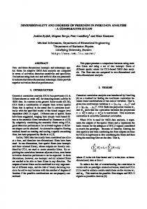
is the observed degrees of freedom (ODF) of the test statistic rK ¸n .h/; similarly, the version of (61) evaluated from the empirical formulas is the EDF. It should be stressed that the difference between the EDF and its asymptotic form may be practically large. Working with the EDF has the advantage of making the distributional results (58) and (60) more closely re ected in nite-sample situations. Therefore, for practical applications of GLR tests, use of the EDF is recommended in place of its asymptotic form given by Fan et al. (2001). 5. SIMULATIONS 5.1 Assessing the Empirical Formulas for Degrees of Freedom This section presents some nite-sample simulation studies. The purposes are two-fold: to assess the extent to which the empirical formulas for DFs approximate their exact values and to illustrate numerical comparisons of different smoothers in which the smoothing parameters are chosen based on the empirical formulas. To simplify the programming, assume that the design is on the interval Ä D [0; 1], so that jÄj D 1 (see Theorem 1) and c.f / D 1 (see Theorem 2). For reasons of computational ef ciency, the Epanechnikov kernel is used throughout the simulations. As an illustration, rst consider the xed uniform design points, xi D .i ¡ :5/=n, i D 1; : : : ; n, in which case the DFs are nonrandom. Determine a and C in the empirical formulas (33)– (35) based on the local linear smoother. With a medium sample size n D 200, the simple least squares estimates of three sets, ¡1 ¡1 T T .h¡1 j ; tr.Sh j //, .hj ; tr.Shj Shj //, and .hj ; tr.2Shj ¡ Shj Shj //, with respect to 20 bandwidths hj , logarithmicallyevenly spaced between :025 and :20, give rise to the estimates of intercept, 1:4531, 1:4603, and 1:4458 and the estimates of slope, :7513, :6033, and :8993. These estimates, combined with (33)–(35) and Table 1, suggest that for p D 1, p C 1 ¡ a ’ 1:45 or a ’ :55, and C ’ 1. The larger the n, the better the approximation provided by the empirical formulas. Using this strategy for local polynomial smoother of other degrees p, the recommended choices for a and C are given in Table 3. Analogously, when the cubic smoothing spline method is applied to the foregoing fxi g, the simple least squares estimates of ¡4 ¡4 T three sets, .¸¡4 j ; tr.S ¸j //, .¸j ; tr.S ¸j S¸ j //, and .¸j ; tr.2S ¸j ¡ ST¸j S¸j //, yield the intercept estimates, 1:0038, 1:0015, and 1:0061, and slope estimates :3533, :2651, and :4416. Thus for q D 2, the choice b D 1 is adopted in (36)–(38). There the range of ¸j values is chosen so as to obtain an agreement in range between the empirical tr.S¸j / and the empirical tr.Shj /. In each panel of Figure 1, the dots denote the actual values of the traces and the centers of the circles denote those evaluated from the empirical formulas. All plots provide convincing evidence that the empirical formulas track the evolution of the DFs as a function of the smoothing parameters nearly perfectly.

618


Table 3. Choices of a and C, in the Empirical Formulas (33)–(35) and (50)–(52), for the pth-Degree Local Polynomial Smoother Design type

p

a

Fixed

0 1 2 3 0 1 2 3

:55 :55 1:55 1:55 :30 :70 1:30 1:70

Random

1 1 1 1

C

:99 1:03 :99 1:03

To see how use of the DF formulas make it easy to compare the amount of smoothing by different types of smoothers, consider Figure 2. This gure displays the local linear t and the cubic smoothing spline t to a sequence of observations Yi at xed-design points xi D .i ¡ :5/=n, simulated from model Yi D m.xi / C ¾ "i ;

i D 1; : : : ; n;

(62)

where m.x/ D :6 C :3 cos.2¼ x/ and "i are independent standard normal random variables. The noise variance ¾ 2 is chosen so that the signal-to-noise ratio (SNR), de ned by varfm.x1 /; : : : ; m.xn /g=¾ 2 , is roughly equal to 4, a median amount of SNR. Figures 2(a) and (b) correspond to the smoothing parameters h and ¸, which are chosen so that the empirical

formulas, (33) for tr.Sh / and (36) for tr.S¸ /, are set at 5 and 11. It can be observed clearly that the empirical DF formulas can produce two types of nonparametric ts comparable in a very simple fashion. Similar plots based on specifying tr.STh Sh / and tr.ST¸ S¸ / have been obtained in Figures 2(c) and (d). Now consider random designs, in which case the observed traces are random quantities and the choices a and C will necessarily differ slightly from their counterparts in the xed design. For the local linear method, the least squares estimates, based on 400 independent U.0; 1/ random variables Xi , give a D :70 and C D 1:03. (These choices are adopted throughout the remaining simulations in random design.) Table 3 collects the choices of a and C for other degrees of the local polynomial regression method. Figure 3 presents typical plots of DFs based on one sample path. These plots show that the empirical formulas capture the observed patterns of the DFs reasonably well. Table 4 summarizes the sample mean and variance of the observed DFs, based on 100 sets of independent samples fXi ; i D 1; : : : ; ng, for n D 400 and 1;000. These summary statistics demonstrate that the average values of the observed DFs are slowly varying with sample size, whereas the variabilities of these random quantities decrease quickly with sample size, and that for xed n, the larger the value of h, the smaller amount of variability in the DFs.

Figure 1. Plots of DFs Versus Smoothing Parameters, Under Fixed Uniform Design. Dots denote the actual values, and centers of circles represent the values using the empirical formulas (33) and (35) for the local linear smoother with a D :55 and C D 1 [(a) and (b)] and (36) and (38) for the cubic smoothing spline with b D 1 [(c) and (d)].


619

Figure 2. Comparison Between Local Linear Fit (dashed curve) and Cubic Smoothing Spline Fit (solid curve) of the Regression Curve in (62), Under Fixed Uniform Design. In (a) and (b), h and ¸ are chosen so that the empirical formulas of tr( Sh ) and tr( S¸ ) are set to be 5 and 11; in (c) and (d), h and ¸ are set based on the empirical formulas of tr( ShT Sh ) and tr ( ST¸ S¸ ).

5.2 Nonparametric Regression Model: Smoothing Parameter Selection This section reports a simulation study done to evaluate the practical performance of the proposed EGCV-based bandwidth selector, as well as some existing bandwidth selectors, for local linear regression. For ease of comparison, consider two sets of regression functions, Example 1: m.x/ D sin.10¼ x/ and

© ª Example 2: m.x/ D .4x ¡ 2/ C 2 exp ¡16.4x ¡ 2/2 ;

in the model Y D m.X/ C ¾ ", with X » U.0; 1/, " » N.0; 1/, and " independent of X. The noise variance ¾ 2 in each case is chosen so that SNR equals 4. A total of 400 random samples are drawn per setting with sample size n D 400. For each of these simulated datasets, four automatically selected bandwidths are computed: hO EGCV ; a bandwidth that minimizes the EGCVI hO GCV ; a bandwidth that minimizes the GCVI

hO FG ; the (global) re ned bandwidth selector of Fan and Gijbels (1995)I

and hO RSW ; the direct plug-in bandwidth selector of Ruppert, Sheather, and Wand (1995): Then h AMISE in (3), the bandwidth asymptotically optimal but in practice unknown, is calculated. The rst three bandwidth selectors are searched over an interval [hmin ; h max ] at a geometric grid of points, hj D C j¡1 hmin , j D 1; 2; : : :, with C > 1. The present implementation uses C D 1:2, hmax D :50, and hmin D max[5=n; max2·j·n fX.j/ ¡X.j¡1/g], where X.1/ ; : : : ; X.n/ denote the order statistics of X1 ; : : : ; Xn . Figure 4 compares the relative errors of these bandwidth selectors to hAMISE . As expected, there is little difference in the behaviors of hO EGCV and hO GCV . In most cases, hO FG and hO RSW tend to oversmooth; this tendency is most pronounced for hO RSW in Example 1. This observation is similar to that obtained from small-sample simulation studies by Lee and Solo (1999), who compared the CVminimizing bandwidth selector with hO FG and hO RSW . Among the four selectors, hO FG has less variation and hO EGCV is closer to the asymptotically optimal bandwidth. Furthermore, numerical experience suggests that hO FG is occasionally unstable when using kernels with bounded support, such as the Epanechnikov kernel; that is, zero values of a matrix trace may occur in the denominator of equation (2.3) of Fan and Gijbels (1995). Figure 4

620


Figure 3. Plots of tr( Sh ) [(a) and (c)] and tr (2 Sh ¡ STh Sh ) [(b) and (d)] Versus Bandwidth h for the Local Linear Method, Under Random Uniform Design. Dots denote the observed values, and centers of circles represent the values using the empirical formulas, (33) and (35), with a D .7 and C D 1.03.

also shows the boxplot error (ASE), P of the averaged squared where ASE D n¡1 niD1 fm O h .Xi / ¡ m.Xi /g2 . In this aspect, the ASEs for all methods exhibit quite similar behavior; however, the ASEs alone may be less informative in distinguishing between bandwidth selectors that produce oversmoothed and undersmoothed ts. 5.3 Varying-Coef cient Model: Fitting Coef cient Functions For the varying-coef cient model, the following example illustrates the performance of the EGCV-based bandwidth selec-

tor in curve tting by the local linear method: Example 1:

Y D sin.3¼ U/X1 C sin.2¼ U/X2 C ¾ ";

(63)

where U follows a uniform distribution on [0; 1] and X1 and X2 are normally distributed with mean 0, unit variance, and correlation coef cient 2¡1=2 . Furthermore, U, .X1 ; X2 /, and " are independent. The noise " follows a standard normal distribution; ¾ is chosen so that the SN ratio is about 4 : 1. First, examine the approximation of the empirical formulas (50)–(52). Generate from model (63) a three-covariate random sample f.Ui ; X1i ; X2i /niD1 g, with each sample consisting of 400

Table 4. Sample Mean and Variance ( %, in brackets) of tr( Sh ), tr ( STh Sh ), and tr(2 Sh ¡ STh Sh ), Based on 100 Independent Samplings, Each of Which Contains n Independent Uniform Random Variables h n 400

Statistic

.0250

.0311

.0387

.0482

.0600

.0747

.0930

.1157

.1440

.1793

tr( Sh )

32:41 (6:44) 26:61 (7:94) 38:21 (5:56) 31:83 (1:01) 25:92 (1:05) 37:74 (1:04)

26:16 (2:69) 21:48 (3:01) 30:83 (2:75) 25:80 (:52) 21:05 (:51) 30:55 (:59)

21:19 (1:35) 17:42 (1:35) 24:97 (1:52) 20:98 (:30) 17:17 (:29) 24:80 (:34)

17:24 (:85) 14:20 (:87) 20:28 (:95) 17:13 (:20) 14:06 (:20) 20:19 (:23)

14:11 (:61) 11:67 (:60) 16:54 (:69) 14:03 (:16) 11:57 (:14) 16:49 (:19)

11:60 (:42) 9:64 (:38) 13:56 (:51) 11:55 (:12) 9:58 (:11) 13:52 (:15)

9:59 (:34) 8:02 (:31) 11:16 (:41) 9:56 (:10) 7:98 (:09) 11:14 (:12)

7:98 (:24) 6:72 (:19) 9:24 (:31) 7:97 (:08) 6:70 (:07) 9:23 (:10)

6:70 (:16) 5:69 (:12) 7:70 (:21) 6:69 (:06) 5:68 (:04) 7:70 (:08)

5:67 (:13) 4:87 (:11) 6:47 (:16) 5:66 (:04) 4:86 (:03) 6:47 (:06)

tr( STh Sh ) tr(2 Sh ¡ STh Sh ) 1;000

tr( Sh ) tr( STh Sh ) tr(2 Sh ¡ STh Sh )


621

O (a) and (b) Boxplots of the relative errors (hO ¡ hAMISE ) =hAMISE . (c) and (d) Boxplots of Figure 4. Comparison of Various h. P Bandwidth Selectors O i ) ¡ m(Xi )g2 . In each panel, the boxplots correspond to (from left to right) hO EGCV , hO GCV , hO FG , and hO RSW . the average squared errors n¡1 niD1 fm(X

observations. Figure 5 compares the exact values of tr.e Sh / and tr.2e Sh ¡ e SThe Sh / with their empirical formulas based on the local linear smoother. As sample size n grows, the overall patterns of the EDFs do resemble those actually observed. Now, 100 independent samples are generated with sample size 400 from (63), and the local linear technique is used to t the varying-coef cient model. The bandwidth is chosen to minimize the EGCV function. Figure 6 depicts the local linear estimates of the varying-coef cient functions a 1 .u/ and a2 .u/ for Example 1, in which the smoothness of a 1 .u/ and the smoothness of a2 .u/ are comparable. In each panel, the solid curves denote the true coef cient functions. Three typically estimated curves are presented, corresponding to the 10th (the dotted curve), 50th (the dashed curve), and 90th (the dashdotted curve) curves, where Ppercentiles among the ASE-based O h .Ui ; Xi / ¡ m.U i ; Xi /g2 . The performance ASE D n¡1 niD1 fm of hO EGCV , when applied to recovering multiple smooth curves in varying-coef cient models, is reasonable. The local polynomial regression method discussed in Section 3 assumes implicitly the similarity between the degrees of smoothness of functions a j .u/, j D 1; : : : ; d. To achieve the optimal rates of convergence for aj .u/ with differing smoothness, the two-step iterative estimation procedure proposed by Fan and Zhang (1999) offers a exible alternative and improvement over the one-step procedure. However, practical implementation of this approach relies on seeking, in the rst-step,

a simple and good pilot bandwidth to estimate a j jointly, and identifying certain functions aj , which are actually signi cantly smoother than the rest of functions and thus need to be reestimated individually in the second step. In such instances, hO EGCV can be easily used in the initial stage for pilot bandwidth; a visual inspection of the preliminary tted curves provides a quick check on the inhomogeneous smoothness across a j .u/. Again, a simple choice of bandwidth in the second-step smoothing is to minimize the EGCV function. Illustrative examples are omitted here. 5.4 Varying-Coef cient Model: Hypothesis Testing The objective in this section is to use simulations to study the discriminatory power of the testing procedure described in Section 4. For illustration, consider a four-covariate varyingcoef cient model, Y D a1 .U/X1 C a2 .U/X2 C a3 .U/X3 C ¾ ":

(64)

Set X3 ´ 1, and let .U; X1 ; X2 ; "/ have the same types of joint distributions as speci ed in the previous section. Suppose that one is interested in the following typical forms of assertions about model (64): .1/

H0 :

a1 .u/ ´ c1 ; a2 .u/ ´ c2 ; a3 .u/ ´ c3

(65)

622


Figure 5. Plots of [(a) and (c)] tr( e Sh ) and [(b) and (d)] tr (2 e Sh ¡ e STh e Sh ) Versus Bandwidth h, When the Local Linear Method is Applied. Dots denote the observed values, and centers of circles represent the values using the empirical formulas (50) and (52), with a D .7 and C D 1.03.

Figure 6. Use of the EGCV-Minimizing Bandwidth Selector for Fitting the Coef cient Functions (a) a1 (u) and (b) a2 (u) in (63). Three typical estimated curves are presented, corresponding to the 10th (dotted curve), the 50th (dashed curve), and the 90th (dashed-dotted curve) percentiles among the ASE-ranked curves. The solid curves denote the true coefcient functions.


623

and .2/ H0

:

a2 .u/ ´ 0;

(66)

.1/

where in H0 the three constants cj are unknown. No other testing procedures deal with the foregoing model-checking problems in varying-coef cient models, so comparisons with published results are impossible. To obtain the critical values and powers of the GLR test statistics rK ¸n .h/, the data are simulated as follows. To test (65), observations are generated from model (64) using the varyingcoef cient functions, a1 .u/ D 1 C µ sin.2¼ u/;

a3 .u/ D 4u.1 ¡ u/µ ¡ 1;

a 2 .u/ D 1=2 ¡ cos.3¼ µu/; µ ¸ 0:

(67)

Analogously, to test (66), the data are generated from model (64) with a1 .u/ D sin.2¼ u/;

a3 .u/ D 4u.1 ¡ u/ ¡ 1;

a2 .u/ D µu 2 ; µ ¸ 0:

(68)

In both cases, µ indexes structural deviations of the alternative models from the null models. Particularly, let µ D 0 characterize the model from which data are simulated under the null hypotheses. Again, the magnitude of ¾ in (64) is determined so that SNR under each null hypothesis equals 4. Note the following remarks about bandwidth selection in model checking. Take the null hypothesis (65), for instance. If a sample of observed data indeed comes from model (64) satisfying this null assumption (linear model), then the optimal bandwidth for local tting of the coef cient functions should be close to in nity, and data-driven bandwidth selectors will lead to a large bandwidth. However, the distributional properties in (58) and (60) rely implicitly on the assumption h ! 0.

Hence the bandwidth well suited for producing visually smooth estimates of the underlying curves may not in general be appropriate for checking model assumptions. Based on this consideration, an empirical bandwidth formula, h ¤ D std.U/ £ n¡2=.4pC5/;

(69)

is proposed for model checking based on the pth degree local polynomial regression. The rate n¡2=.4pC5/ was given by Fan et al. (2001); in practice, the standard deviation of the covariate U can be simply replaced by its sample standard deviation. 5.4.1 Large Datasets. First, methodologies for processing large datasets are developed. Experience indicates that under the null hypotheses, the sampling distribution of the test statistic, rK ¸n .h¤ /, is close to a chi-squared distribution, 2 ÂEDF C2 , where EDF represents the empirical degrees of freedom for hypothesis testing, de ned at the end of Section 4. To see this, simulate, from the null hypotheses (65) and (66), 400 random samples each of size 400. Figure 7(a) and Figure 8(a) plot the kernel density estimates (Fan and Gijbels 1996, p. 47) of frK ¸n .h¤ /g, for (65) and (66). For comparison, two reference density functions are also included:p the normal density with mean EDF and standard deviation 2 EDF 2 and the chi-squared density ÂEDF C2 . Table 5 compares the simulated rejection rates of rK ¸n .h¤ / exceeding the 100.1 ¡ ®/th percentiles of the reference distributions. Note that the chi-squared approximation gives better agreement with the nominal type-I errors than does the normal approximation. Moreover, using EDF instead of ODF in the parameters of the reference distributions makes little difference in approximating the tail distribution of rK ¸n .h ¤ /, but has the added merit of being quickly implemented. To measure the GLR test’s ability to detect departures from the null, the following power studies were performed.

Figure 7. (a) Kernel density estimate of the test statistics, rK ¸ n (h¤ ), under the null hypothesis (65), p based on 400 random samples each of size 400. The solid curve represents kernel density estimate; the dotted curve, density of N(EDF , 2EDF ); and the dashed curve, density of 2 ÂEDF C2 . (b) Estimated power curves when the data are simulated from (67). The solid curve is based on the simulated null critical values, and the 2 dashed curve is based on the percentile of ÂEDF C2 . The bottom dotted line denotes the nominal level of signi cance.

624


Figure 8. Same as Figure 7, Except That (a) Shows the Null Hypothesis (66) and in (b) the Data Are Simulated From (68).

A total of 400 independent samples were simulated from the alternative models indexed by µ , with each sample containing 400 observations; for simplicity, 10 values of µ evenly spaced on an interval [0; :15] with (67) and [0; :5] with (68) were considered. At a nominal level 5%, the empirical powers are estimated through simulation by the proportion of observed test statistics rK ¸n .h¤ /, across 400 samples, exceeding the 95th 2 percentile of the ÂEDF C2 distribution. For comparison, also included is the rate of the observed test statistics exceeding their 95th sample percentile, under the null, across 400 samples. Figures 7(b) and 8(b) display the estimated power curves. It is clear that the GLR tests are powerful, besides holding their correct sizes. Simulation studies of model checking with small datasets, via the bootstrap procedure, are omitted here. 6. DISCUSSION This article has provided a simple, yet exible extension of the criterion based on GCV, termed EGCV, for smoothing pa-

rameter selection in nonparametric regression. By using an empirical formulas of DFs, the computational burden associated with smoothing large datasets is improved considerably, and the procedure for model checking is also easier to carry out. It is hoped that the methodology presented here will be useful in mining large collections of data. In closing, several points bear mentioning. First, an application to bandwidth selectors based on principles other than CV or GCV would also be valuable. Hurvich, Simonoff, and Tsai (1998) used an improved Akaike information criterion, to which the empirical formulas of DFs proposed here can also apply. Second, if there is a clear indication P that the design is nonuniform, then the data-based form, n¡1 niD1 f ¡1 .Xi /, could be used directly in place of its asymptotic form, jÄj, in the empirical formulas (33)–(35); refer to (A.10) and (A.18) for further derivational details. In such instances, if f is unknown, then those f .Xi / can be replaced by their kernel density estimates, which are computationally far more economic than evaluating the actual traces, but will surely improve the nite-sample performance of the empirical approximations.Indeed, experiments

Table 5. Simulated Rejection Rates of the Test Statistics, Based on 400 Random Samples of Size n D 400, (1) (2) From Null Hypotheses H0 and H0 . The signi cance levels are ® D :01; :025; :05 ; :10 Null (1) H0

(2)

H0

Test statistic rK ¸ n

(h¤ )

rK ¸n (h¤ )

Reference distribution p N(EDF; p2EDF) N(ODF; 2ODF) p N(EDF C 2; p2 (EDF C 2)) N(ODF C 2; 2 (ODF C 2))

® D :01

Rejection rate at level ® ® D :025 ® D :05

® D :10

2 ÂEDFC2 2 ÂODFC2

.0250 .0250 .0125 .0150 .0075 .0075

.0500 .0550 .0300 .0300 .0200 .0200

.0750 .0875 .0550 .0550 .0400 .0475

.1375 .1425 .0950 .0975 .0900 .0950

2 ÂEDFC2 2 ÂODFC2

.0450 .0450 .0200 .0200 .0075 .0050

.0725 .0750 .0375 .0375 .0200 .0200

.1150 .1175 .0575 .0575 .0450 .0450

.1700 .1700 .0950 .0925 .0850 .0875

p N(EDF; p2EDF) N(ODF; 2ODF) p N(EDF C 2; p2 (EDF C 2)) N(ODF C 2; 2 (ODF C 2))


with this modi cations have yielded results comparable with those in the uniform design. Third, if f is other than uniformity but known, then the higher-order approximationsgiven in (A.9) and (A.17) may perform better than those in (A.10) and (A.18). On the other hand, even a decent approximation, as simple as the rst-order empirical formulas, is likely to be satisfactory. Fourth, some robust procedures may be applied before the empirical formulas are used; for example, remove a few design observations at the edges of the sample space. This preprocessing of the raw data before the analyses are performed is also common in other contexts of statistical applications. APPENDIX: PROOFS OF MAIN RESULTS Condition (A) (A1) The design variable X has a bounded support Ä; the marginal density f of X is Lipschitz continuous and bounded away from 0. (A2) m.x/ has the continuous p C 1th derivative in Ä. (A3) The kernel function K.t/ is a symmetric probability density function with bounded support and is Lipschitz continuous. (A4) 0 < E." 4 / < 1.

Condition (A¤ ) is similar to condition (A), except that (A1) is replaced by (A1 ¤ ).

(A1 ¤ ) The design observations X i D xi , i D 1; : : : ; n, are generated by xi D F ¡1 ..i ¡ :5/=n/, where F has a probability density function f with a bounded support Ä; f is Lipschitz continuous and bounded away from 0.

625

Proof. To show part 1, it is seen that fSh .i; j/g2 D eT1 fSn .Xi /g¡1 f1; .Xj ¡ Xi /; : : : ; .Xj ¡ X i /p gT £ f1; .Xj ¡ Xi /; : : : ; .Xj ¡ X i / p g £ fSn .X i /g¡1 e1 Kh2 .X j ¡ Xi / · eT1 fSn .Xi /g¡1 f1; .Xj ¡ Xi /; : : : ; .Xj ¡ X i /p gT £ f1; .Xj ¡ Xi /; : : : ; .Xj ¡ X i / p g

Pn

2 T ¡1 jD1 fSh .i; j/g · e1 fSn .Xi /g e1 Kh .0/ D Sh .i; i/. Pn X ¡x To show part 2, recall that jD1 .X j ¡ x/ k W 0n .x; jh / D I.k D 0/

and thus

holds for any integer k D 0; 1; : : : ; p (Fan and Gijbels 1996, p. 103). Applying this result and the binomial expansion leads to n X jD1

n X k ³ ´ ± X ¡x² X ± X ¡ x² k j j D Xjk W0n x; .Xj ¡ x/` xk¡` W 0n x; h h ` jD1 `D0

D

Condition (C) (C1) The covariate U has a bounded support Ä; the marginal density fU of U is Lipschitz continuous and bounded away from 0. (C2) aj .u/, j D 1; : : : ; d, has the continuous p C 1th derivative in Ä. (C3) The kernel function K.t/ is a symmetric probability density function with bounded support and is Lipschitz continuous. (C4) 0 < E." 4 / < 1. (C5) The matrix E.XXT jU D u/ is positive de nite for each u 2 Ä, and each entry is Lipschitz continuous. Condition (C¤ ) is similar to condition (C), except that (C1) is replaced by (C1¤ ). (C1 ¤ ) The covariate observations U i D ui are generated by ui D ¡1 F U ..i ¡ :5/=n/, where FU has a probability density function fU with a bounded support Ä; fU is Lipschitz continuous and bounded away from 0.

tr.S Th Sh / D

Lemma P A.1. 1. For a nonnegative kernel K satisfying K.0/ D supx K.x/, njD1 fSh .i; j/g2 · S h .i; i/ for i D 1; : : : ; n, and thus 0 · Sh .i; i/ · 1, and jSh .i; j/j · 1 for i 6D j. 2. For any integer k D 0; 1; : : : ; p, Sh .X 1k ; : : : ; Xnk /T D .X1k ; : : : ; k X n /T . Thus for any matrix P whose column space is generated by the vectors .X1k ; : : : ; X nk /T , k D 0; 1; : : : ; p, it follows that Sh P D P and .STh C Sh ¡ STh Sh /` P D P for integers ` ¸ 0.

`D0

`

xk¡`

n X jD1

± X ¡ x² j .X j ¡ x/ ` W 0n x; h

n X n X iD1 jD1

fS h .i; j/g2 · tr.Sh /

(A.1)

holds under the kernel-mode condition. The second part of Lemma A.1 asserts that 1 is an eigenvalue of S h corresponding to a number p C 1 of distinct eigenvectors. Let ¸i .Sh /, i D 1; : : : ; n, denote all of the eigeninequality (Marcus and Minc 1964, p. 142) values of S h . Then Schur’s P says that tr.STh Sh / ¸ niD1 j¸i .Sh /j2 ¸ pC 1. Henceforth, this inequality, together with (A.1) and trf.In ¡ Sh / T .In ¡ Sh /g > 0, implies the expected results. Proof of Theorem 1 For each i D 1; : : : ; n, because the ith row of X.X i / is eT1 , and the ith diagonal entry of W.Xi / is K h .0/, Sn .X i / D K h .0/e1 eT1 C Ai can be rewritten, where the .`; r/th entry of the matrix Ai is given by X Ai .`; r/ D .X k ¡ Xi /`Cr¡2 Kh .Xk ¡ Xi /; k: k6Di

`; r D 1; : : : ; p C 1: Set dij D

X j ¡Xi ¡1 D A¡1 ¡ i h . Thus the use of fSn .Xi /g

together with (10) and (11), implies S h .i; j/ D

Proof of (14) This proof begins with Lemma A.1.

k ³ ´ X k

D xk : P P X ¡X Thus for each i D 1; : : : ; n, njD1 Sh .i; j/X jk D njD1 X jk W0n .Xi , j h i / D X ik . Lemma A.1 nishes. To show (14), observe from the rst part of Lemma A.1 that

Condition (B) The design points xi , i D 1; : : : ; n, are generated from a continuous and strictly positive density f , on R xa nite interval [0; 1] without loss of generality, through the relation 0 i f .x/ dx D .i ¡ :5/=n.

£ Kh .Xj ¡ Xi /fSn .Xi /g¡1 e1 Kh .0/;

where

(A.2)

T ¡1 A¡1 i e 1 e 1 Ai h=K.0/CeT1 A¡1 i e1

Bij ; h=K.0/ C B ii

,

(A.3)

p

T Bij D eT1 A¡1 i H.1; dij ; : : : ; dij / K.dij /=K.0/;

i; j D 1; : : : ; n:

(A.4)

Writing fi D f .X i /, fi0 D f 0 .Xi /, fi00 D f 00 .Xi /, gi1 D fi0 =fi , and gi2 D 2¡1 .fi00 =fi /, then the higher-order Taylor expansion of Ai .`; r/, `; r D 1; : : : ; p C 1, leads to

Ai D .n ¡ 1/fi H.S C hgi1e S C h2 gi2 S/Hf1 C oP .1/g;

(A.5)

626


SD where oP .1/ is uniform in i D 1; : : : ; n (abbreviated as Ui), e .¹`Cr¡1 /1·`; r·pC1 , and S D .¹`Cr /1·`; r·pC1 . Denote M 1 D S¡1e SS¡1 , M2 D S ¡1e SS¡1e SS¡1 , and M 3 D S¡1 SS¡1 ; then

in which this oP .1/ can also be IjUi, under the smoothness assumption on f . Similar to the derivation of (A.5), X p p .1; dij ; : : : ; dij /T .1; dij ; : : : ; dij /K 2 .dij /

A¡1 i D

j: j6Di

1 H ¡1 fS¡1 ¡ hgi1 M1 C h2 .g2i1 M2 ¡ gi2 M3 /gH ¡1 .n ¡ 1/fi £ f1 C oP .1/g;

(A.6)

Ui. Set Ke.t/ D eT1 M1 .1; t; : : : ; t p /T K.t/, K .t/ D eT1 M2 .1; t; : : : ; t p /T K.t/, and K .t/ D eT1 M3 .1; t; : : : ; t p /T K.t/. Equations (A.4) and (A.6), together with the fact that Ke.0/ D 0, give Bii D

1 fK .0/ C h2 .g2i1 K ¡ gi2 K /.0/g .n ¡ 1/K.0/fi

£ f1 C oP .1/g;

D .n ¡ 1/hfi .S ¤ C hgi1 Se¤ C h2 gi2 S¤ /f1 C oP .1/g;

j: j6Di

(A.7)

X

Ui, an immediate consequence of which is

j: j6Di

X

(A.8)

j: j6Di

n X

and

K .0/ C h2 .g2i1 K ¡ gi2 K /.0/

.n ¡ 1/hfi C fK .0/ C h2 .g2i1 K ¡ gi2 K /.0/g iD1

£ f1 C oP .1/g ³X ´ n K .0/ D fi ¡1 f1 C oP .1/g: .n ¡ 1/h

(A.9) (A.10)

X j: j6Di

iD1

fSh .i; i/g2 C

XX

£ f1 C oP .1/g;

fSh .i; j/g2 :

(A.11)

1·i6Dj·n

D OP f.nh2 /¡1 g:

(A.12)

1 fK .dij / ¡ hgi1 Ke.dij / .n ¡ 1/K.0/fi

D

n X [K ¤ K .0/ C h2 fg2i1 `1 .K/ ¡ gi2 `2 .K/g].n ¡ 1/hfi iD1

[.n ¡ 1/hfi C fK .0/ C h2 .g2i1 K ¡ gi2 K /.0/g]2

£ f1 C oP .1/g ³ n ´ K ¤ K .0/ X ¡1 D fi f1 C oP .1/g: .n ¡ 1/h

(A.17) (A.18)

iD1

C h2 .g2i1 K ¡ gi2 K /.dij /gf1 C oP .1/g;

(A.13)

where the term oP .1/ is independent of j and uniform in i D 1; : : : ; n (abbreviated as IjUi). It can be deduced that from (A.3), (A.7), and (A.13), K .dij / ¡ hgi1 Ke.dij / C h2 .g2i1 K ¡ gi2 K /.dij / .n ¡ 1/fi C fK .0/ C h2 .g2i1 K ¡ gi2 K /.0/g £ f1 C oP .1/g;

This, together with (A.11) and (A.12), nishes the proof of the second part. Proof of the third part is trivial from the rst two parts. For xed designs, the proofs follow arguments analogous to the foregoing. For example, (A.5) and (A.15) follow from the theory of Riemann sums, with oP .1/ replaced by o.1/. Proof of Theorem 2

(A.14)

IjUi. For the numerator of (A.14), fK .dij / ¡ hgi1 Ke.dij / C h2 .g2i1 K ¡ gi2 K /.dij /g2 D K 2 .dij / ¡ 2hgi1 K Ke.dij /

fSh .i; j/g2

iD1 j: j6Di

Consider the second additive term of (A.11). According to (A.4) and (A.6), it holds that

Sh .i; j/ D

(A.16)

again due to the fact K ¤ Ke.0/ D 0, where `1 .K/ D 2K ¤ K .0/ C Ke ¤ Ke.0/ ¡ 2e T1 S¡1 Se¤ M1 e1 and `2 .K/ D 2K ¤ K .0/ ¡ eT1 S¡1 S¤ S¡1 e1 . Applying (A.14) and (A.16), it can be observed that n X X

n X

K 2 .0/ fS h .i; i/g2 D f1 C oP .1/g .n ¡ 1/2 h2 fi2 iD1 iD1

Bij D

K K .dij / D .n ¡ 1/hfi K ¤ K .0/f1 C oP .1/g;

D .n ¡ 1/hfi [K ¤ K .0/ C h2 fg2i1 `1 .K/ ¡ gi2 `2 .K/g]

For the rst additive term of (A.11), from (A.8), n X

K K .dij / D .n ¡ 1/hfi K ¤ K .0/f1 C oP .1/g;

Ui. Hence, uniformly in i, X fK .dij / ¡ hgi1 Ke.dij / C h2 .g2i1 K ¡ gi2 K /.dij /g2

This nishes the proof of the rst part. For tr.STh Sh /, the fact is that tr.STh S h / D

Ke2 .dij / D .n ¡ 1/hfi Ke ¤ Ke.0/f1 C oP .1/g;

j: j6Di

iD1

n X

K Ke.dij / D .n ¡ 1/hfi fhgi1 eT1 S ¡1 Se¤ M 1 e1 gf1 C oP .1/g;

j: j6Di

Ui, and therefore, tr.Sh / D

£ f1 C oP .1/g;

X

K .0/ C h2 .g2i1 K ¡ gi2 K /.0/ Sh .i; i/ D .n ¡ 1/hfi C fK .0/ C h2 .g2i1 K ¡ gi2 K /.0/g £ f1 C oP .1/g;

(A.15)

Ui, where S ¤ D .ºiCj¡2 /1·i; j·pC1 , Se¤ D .ºiCj¡1 /1·i; j·pC1, and S ¤ D .ºiCj /1·i; j·pC1 . Analogously, using (17), eT1 S¡1 Se¤ S¡1 e1 D 0, and eT1 S¡1 S¤ M1 e 1 D K ¤ Ke.0/ D 0, it can be deduced that X K 2 .dij / D .n ¡ 1/hfi fK ¤ K .0/ C h2 gi2 eT1 S¡1 S¤ S¡1 e1 g

C h2 fg2i1 .2K K C Ke2 / ¡ 2gi2 K K g.dij /f1 C oP .1/g;

The proof of Theorem 2 depends on two lemmas. The proof of Lemma A.2 was given by Ramil Novo and González Manteiga (2000). R C1 Lemma A.2. Let K.x/ D .2¼ / ¡1 ¡1 .1 C t 2q / ¡1 exp.¡itx/ dt, r

z }| { with q D 1; 2; : : : . Denote by K ¤ ¢ ¢ ¢ ¤ K .x/ the r-times convolution product of K.x/. Then r Z C1 z }| { 1 2q ¡r .1 C t / dt DK ¤ ¢ ¢ ¢ ¤ K .0/; 2¼ ¡1

r D 1; 2; : : : :


In particular, .2¼ /¡1

R C1

` D 1; 2; : : : .

¡1

627 `

.1 C t 2q /¡2` dt D

R z }| { 2 .K ¤ ¢ ¢ ¢ ¤ K/ .x/ dx for

Ui, and tr.e Sh / D

R C1 Lemma A.3. Let K.x/ D .2¼ / ¡1 ¡1 .1 C t2q /¡1 exp.¡itx/ dt. Set R1 c.f / D 0 f .t/ 1=.2q/ dt. Then for q ¸ 2, as n ! 1, ¸ ! 0, and n¸ !

1, it holds that

tr.S r¸/ D q C ¸¡1=.2q/c.f /.2¼ /¡1

Z C1 ¡1

.1 C t2q /¡r dt f1 C o.1/g; r ¸ 1:

(A.19)

P Proof. From (25), rst observe that tr.Sr¸ / D q C njDqC1 .1 C ¸°jn /¡r , for integers r ¸ 1. Speckman (1981) showed that if q ¸ 2, then °jn D j2q c0 f1 C o.1/g for 1 · j · n, where c0 D R1 ¼ 2q f 0 f .t/ 1=.2q/ dtg ¡2q , and the o.1/ term is uniform for j D o.n2=5 /. Combining this result, it can be deduced that X X .1 C ¸°jn /¡r D .1 C ¸c0 j2q / ¡r f1 C o.1/g qC1·j·n3=.4q/

qC1·j·n3=.4q/

D .¸c0 /¡1=.2q/

Z 1 0

dt .1 C t2q /r

f1 C o.1/g:

On the other hand, the sequence f°jn gnjD1 is nondecreasing, and therefore ° jn ¸ O.n3=2 / for j ¸ n3=.4q/ , so that X .1 C ¸° jn /¡r · Ofn.n3=2 ¸/¡r g:

The upper bound in (A.20) is Rthus of¸¡1=.2q/ g if r ¸ 2. Hence C1 tr.Sr¸ / D q C ¸¡1=.2q/c.f /.2¼ / ¡1 ¡1 .1 C t2q /¡r dt f1 C o.1/g for r ¸ 2. For r D 1, a similar expression for tr.S¸ / was given by Eubank (1988, p. 327). This nishes the proof of Lemma A.3. To obtain the asymptotic representations of tr.S¸ / and tr.S2¸ /, in terms of Silverman’s kernel function K, a direct application of Lemma A.2 to Lemma A.3 leads to the desired conclusions. Proof of Theorem 3 Sn .Ui / D K h .0/.e1 Xi /.eT1 First, according to the de nition (41), e P T Xi / C A i , where A i D k: k6Di Z k .Ui /fZk .Ui /g T Kh .Uk ¡ U i /. Set U j ¡Ui h . Thus the use of

© ª¡1 e Sn .U i / D A¡1 i ¡

T T ¡1 A¡1 i .e1 Xi /.e1 Xi /Ai

h=K.0/ C .eT1 XTi /A¡1 i .e1 Xi / together with (44) and (45), implies that e Sh .i; j/ D where

Bij ; h=K.0/ C Bii

;

(A.21)

p

T Bij D .eT1 XTi /A¡1 i .H Id /f.1; dij ; : : : ; dij / Xj gK.dij /=K.0/;

i; j D 1; : : : ; n:

(A.22)

It can be shown via some standard arguments that

Ai D .n ¡ 1/f.HSH/ 0.Ui /gf1 C oP .1/g

(A.23)

and ¡1 ¡1 ¡1 ¡1 ¡1 A¡1 i D .n ¡ 1/ [.H S H / f0.U i /g ]f1 C oP .1/g; (A.24)

Ui, where 0.u/ D fU .u/E.XXT jU D u/. This results in Bii D e Sh .i; i/ D

K .0/ XT f0.Ui /g ¡1 Xi f1 C oP .1/g; .n ¡ 1/K.0/ i K .0/XTi f0.Ui /g¡1 Xi

.n ¡ 1/h C K .0/XTi f0.Ui /g¡1 Xi

f1 C oP .1/g;

e Sh .i; i/

iD1

³X ´ n K .0/ XTi f0.U i /g¡1 Xi f1 C oP .1/g; (A.27) .n ¡ 1/h iD1

which, combined with EfXTi f0.Ui /g¡1 Xi g D djÄj, nishes the proof of the rst part. Sh /. According to (A.22) and (A.24), it can be Now consider tr.e STh e deduced that Bij D and e Sh .i; j/ D

K .dij / XT f0.Ui /g ¡1 Xi f1 C oP .1/g .n ¡ 1/K.0/ i K .dij /XTi f0.U i /g¡1 Xj

.n ¡ 1/h C K .0/XTi f0.Ui /g¡1 Xi

(A.28)

f1 C oP .1/g;

(A.29)

IjUi. Veri cation of X K 2 .dij /Xj XTj D .n ¡ 1/h0.Ui /K ¤ K .0/f1 C oP .1/g; j: j6Di

Ui, implies that (A.20)

n3=.4q/ 0, O h; ¡i .U i ; Xi / D m O h; ¤i.U i ; Xi /. This equality in turn yields indicate m m O h; ¡i .U i ; Xi / D m O h; ¤i .Ui ; Xi / X e D Sh .i; j/Yj C e O h; ¡i .U i ; Xi / Sh .i; i/m 1·j·n: j6Di

D

n X jD1

e Sh .i; j/Yj C e O h; ¡i .Ui ; Xi / ¡ Yi g Sh .i; i/fm

Dm O h .Ui ; Xi / C e O h; ¡i .Ui ; Xi / ¡ Yi g: Sh .i; i/fm

O h;¡i .U i ; Xi / D Y i ¡ m O h .U i ; Xi / C e O h;¡i £ Hence Yi ¡ m Sh .i; i/fYi ¡ m O h;¡i .Ui ; Xi / D fYi ¡ .Ui ; Xi /g, which leads to the stated result, Y i ¡ m m O h .U i ; Xi /g=f1 ¡ e Sh .i; i/g, for i D 1; : : : ; n. [Received May 2002. Revised January 2003.]

REFERENCES Allen, D. M. (1974), “The Relationship Between Variable and Data Augmentation and a Method of Prediction,” Technometrics, 16, 125–127. Buckley, M. J., Eagleson, G. K., and Silverman, B. W. (1988), “The Estimation of Residual Variance in Nonparametric Regression,” Biometrika, 75, 189– 200. Cleveland, W., and Devlin, S. (1988), “Locally Weighted Regression: An Approach to Regression Analysis by Local Fitting,” Journal of the American Statistical Association, 83, 596–610. Cleveland, W. S., Grosse, E., and Shyu, W. M. (1992), “Local Regression Models,” in Statistical Models in S, eds. J. M. Chambers and T. J. Hastie, Paci c Grove, CA: Wadsworth/Brooks Cole, pp. 309–376. Craven, P., and Wahba, G. (1979), “Smoothing Noisy Data With Spline Functions,” Numerische Mathematik, 31, 377–403. Cummins, D. J., Filloon, T. G., and Nychka, D. (2001), “Con dence Intervals for Nonparametric Curve Estimates: Toward More Uniform Pointwise Coverage,” Journal of the American Statistical Association, 96, 233–246. Demmler, A., and Reinsch, C. (1975), “Oscillation Matrices With Spline Functions,” Numerische Mathematik, 24, 375–382. Eubank, R. L. (1984), “The Hat Matrix for Smoothing Spline,” Statistics and Probability Letters, 2, 9–14. (1988), Spline Smoothing and Nonparametric Regression, New York: Marcel Dekker. Fan, J., and Gijbels, I. (1995), “Data-Driven Bandwidth Selection in Local Polynomial Fitting: Variable Bandwidth and Spatial Adaptation,” Journal of the Royal Statistical Society, Ser. B, 57, 371–394. (1996), Local Polynomial Modeling and Its Applications, London: Chapman & Hall. Fan, J., Zhang, C. M., and Zhang, J. (2001), “Generalized Likelihood Ratio Statistics and Wilks Phenomenon,” The Annals of Statistics, 29, 153–193. Fan, J., and Zhang, W. Y. (1999), “Statistical Estimation in Varying Coef cient Models,” The Annals of Statistics, 27, 1491–1518.

Gasser, T., Kneip, A., and Köhler, W. (1991), “A Flexible and Fast Method for Automatic Smoothing,” Journal of the American Statistical Association, 86, 643–652. Green, P. J., and Silverman, B. W. (1994), Nonparametric Regression and Generalized Linear Models: a Roughness Penalty Approach, London: Chapman & Hall. Härdle, W., Hall, P., and Marron, J. S. (1992), “Regression Smoothing Parameters That Are Not Far From Their Optimum,” Journal of the American Statistical Association, 87, 227–233. Hastie, T. J., and Tibshirani, R. J. (1990), Generalized Additive Models, London: Chapman & Hall. (1993), “Varying-Coef cient Models” (with discussion), Journal of the Royal Statistical Society, Ser. B, 55, 757–796. Hoover, D. R., Rice, J. A., Wu, C. O., and Yang, L. P. (1998), “Nonparametric Smoothing Estimates of Time-Varying Coef cient Models With Longitudinal Data,” Biometrika, 85, 809–822. Hurvich, C. M., Simonoff, J. S., and Tsai, C.-L. (1998), “Smoothing Parameter Selection in Nonparametric Regression Using an Improved Akaike Information Criterion,” Journal of the Royal Statistical Society, Ser. B, 60, 271–293. Lee, T. C. M., and Solo, V. (1999), “Bandwidth Selection for Local Linear Regression: A Simulation Study,” Computational Statistics, 14, 515–532. Li, K.-C. (1985), “From Stein’s Unbiased Risk Estimates to the Method of Generalized Cross-Validation,” The Annals of Statistics, 13, 1352–1377. (1986), “Asymptotic Optimality of CL and Generalized CrossValidation in Ridge Regression With Application to Spline Smoothing,” The Annals of Statistics, 14, 1101–1112. Marcus, M., and Minc, H. (1964), A Survey of Matrix Theory and Matrix Inequalities, Boston: Allyn and Bacon. Müller, H. G. (1987), “Weighted Local Regression and Kernel Methods for Nonparametric Curve Fitting,” Journal of the American Statistical Association, 82, 231–238. (1988), Nonparametric Regression Analysis of Longitudinal Data (Lecture Notes in Statistics, Vol. 46), Berlin: Springer-Verlag. Müller, H. G., and Prewitt, K. A. (1993), “Multiparameter Bandwidth Processes and Adaptive Surface Smoothing,” Journal of Multivariate Analysis, 47, 1– 21. Ramil Novo, L. A., and González Manteiga, W. (2000), “F-Tests and Regression ANOVA Based on Smoothing Spline Estimators,” Statistica Sinica, 10, 819–837. Ramsay, J. O., and Silverman, B. W. (1997), Functional Data Analysis, New York: Springer-Verlag. Reinsch, C. (1967), “Smoothing by Spline Functions,” Numerische Mathematik, 10, 177–183. Rice, J. (1984), “Bandwidth Choice for Nonparametric Regression,” The Annals of Statistics, 20, 712–736. Ruppert, D., Sheather, S. J., and Wand, M. P. (1995), “An Effective Bandwidth Selector for Local Least Squares Regression,” Journal of the American Statistical Association, 90, 1257–1270. Ruppert, D., Wand, M. P., Holst, U., and Hössjer, O. (1997), “Local Polynomial Variance-Function Estimation,” Technometrics, 39, 262–273. Silverman, B. W. (1984), “Spline Smoothing: the Equivalent Variable Kernel Method,” The Annals of Statistics, 19, 898–916. Speckman, P. (1981), “The Asymptotic Integrated Mean Squared Error for Smoothing Noisy Data by Spline Functions,” unpublished manuscript, University of Missouri, Dept. of Statistics. Stanton, R. (1997), “A Nonparametric Model of Term Structure Dynamics and the Market Price of Interest Rate Risk,” Journal of Finance, 52, 1973–2002. Stone, C. (1984), “An Asymptotically Optimal Window Selection Rule for Kernel Density Estimates,” The Annals of Statistics, 12, 1285–1297. Stone, M. (1974), “Cross-Validatory Choice and Assessment of Statistical Predictions” (with discussion), Journal of the Royal Statistical Society, Ser. B, 36, 111–147. Wahba, G. (1990), Spline Models for Observational Data, Philadelphia: Society for Industrial and Applied Mathematics. Wand, M. P., and Jones, M. C. (1995), Kernel Smoothing, London: Chapman & Hall. Wong, W. H. (1983), “On the Consistency of Cross-Validation in Kernel Nonparametric Regression,” The Annals of Statistics, 11, 1136–1141. Ye, J. M. (1998), “On Measuring and Correcting the Effects of Data Mining and Model Selection,” Journal of the American Statistical Association, 93, 120–131.

Calibrating the Degrees of Freedom for Automatic Data ... - CiteSeerX

Calibrating the Degrees of Freedom for Automatic Data ... - CiteSeerX

Suggest Documents

DEGREES OF FREEDOM OF EQUIPMENT AND ... - CiteSeerX

DIMENSIONALITY AND DEGREES OF FREEDOM IN ... - CiteSeerX

queue size follows degrees of freedom - CiteSeerX

What Are Degrees of Freedom? - CiteSeerX

Freedom of Choice? Degrees of Freedom?

Freedom of Choice? Degrees of Freedom?

Freedom of Choice? Degrees of Freedom?

On the Degrees of Freedom of the Compound MIMO ... - CiteSeerX

The Generalized Degrees of Freedom of the

Degrees of Freedom - Semantic Scholar

On the Degrees of Freedom of MISO Broadcast Channels ... - CiteSeerX

Degrees-of-Freedom Analysis of Case Data in Business Marketing ...

Improving the Estimation of the Degrees of Freedom for

Sum Degrees-of-Freedom of Two-Unicast Wireless ... - CiteSeerX

Recruitment of Degrees of Freedom Stabilizes Coordination - CiteSeerX

Dynamic analysis of a three-degrees-of-freedom in ... - CiteSeerX

Sum Degrees-of-Freedom of Two-Unicast Wireless ... - CiteSeerX

Degrees of Freedom Region for the MIMO X Channel - arXiv.org

Evidence for nonhadronic degrees of freedom in the transverse mass ...

Degrees of freedom and optimal operation of simple heat ... - CiteSeerX

Achievable Degrees of Freedom for the Two-Cell Two ...

Role of kinematic degrees of freedom in frog jumping - CiteSeerX

DEGREES OF FREEDOM OF ARBITRARILY HIGHER-DERIVATIVE ...

ERGOS: Multi-degrees of Freedom and Versatile Force ... - CiteSeerX