Calibration and Synchronization of a Robot-Mounted ... - CiteSeerX

IEEE Int. Conf. on Robotics and Automation ICRA2005, Barcelona, Spain, April 2005

Calibration and Synchronization of a Robot-Mounted Camera for Fast Sensor-Based Robot Motion Friedrich Lange and Gerd Hirzinger Deutsches Zentrum f¨ur Luft- und Raumfahrt e. V. (DLR) Oberpfaffenhofen, D-82234 Weßling, Germany http://www.robotic.dlr.de/Friedrich.Lange/

Abstract— For precise control of robots along paths which are sensed online it is of fundamental importance to have a calibrated system. In addition to the identification of the sensor parameters - in our case the camera calibration we focus on the adaptation of parameters that characterize the integration of the sensor into the control system or the application. The most important of such parameters are identified best when evaluating an application task, after a short pre-calibration phase. The method is demonstrated in experiments in which a robot arm follows a curved line at high speed. Index Terms— visual servoing, adaptation, calibration, self calibration, synchronization

I. I NTRODUCTION We discuss the task of an off-the-shelf industrial robot manipulator which has to be servoed along unknown curved lines as e.g. cables or edges of workpieces (see Fig. 1). This sample task stands for a variety of applications as the spraying of the glue for a sealing or the cutting of parts using a laser. Such visual servoing task have to be realized at high speed. Therefore in addition to an appropriate camera we need a special control approach. In former papers, [1], [2], the authors proposed a universal sensor control architecture (see Fig. 3). This approach consists of two levels: In the lower level a predictive positional control is implemented. This control completes the control setup provided by the robot manufacturer by

Fig. 1. The task: Refinement of the robot path so that the cable remains in the image center

adding an adaptive feedforward controller. The upper level defines the desired trajectory using image data. The interface between the two levels is not only represented by the current desired and actual pose of the tool center point (tcp). In addition the part of the desired trajectory which has to be executed in the next sampling steps is provided. This enables the feedforward controller to realize an ideal robot which accurately follows the desired path without delay. The desired trajectory is determined by a camera which is mounted near the tcp. Since the positions of sensed object points xs are acquired with respect to the camera pose, the components of a desired position of the tcp xd(k+i) result from the actual position of the camera xc(k) at the time instant k of the exposure and from image points which can be matched to object points corresponding to sampling step (k +i) (see Fig. 2). Assuming that the camera is always aligned with the world system this yields xs(k+i) = xc(k) + c(k) xs(k+i) ,

(1)

where an upper left index denotes the system to which the point is related. This means that c(k) xs(k+i) is the difference between the point xs(k+i) and the camera. c(k) xs(k+i) is computed from the coordinates of image points measured without error, and from the given distance of the object points in time step (k + i). The desired position xd(k+i) is then computed from xs(k+i) by adding the desired distance.

Fig. 2. View of the robot mounted camera: The line is visible for the current time instant (image center) and for future sampling steps

Fig. 3. Control architecture with positional control as lower level (green) and the determination of the desired path as upper level. (Bold face lines include predicted future values.)

Degrees of freedom of xd which cannot be determined by image information are given in terms of a reference path. Adaptation of the feedforward controller of the lower level is possible using predefined paths, i.e. without using the vision system. For this task the goal is to minimize the difference between the actual robot joint angles which can be internally measured and the desired joint values given by the reference path [3], [4]. Unfortunately, adaptation of the upper level und thus optimization of the total system cannot be easily reached. According to Gangloff and de Mathelin [5] the reachable path accuracy when tracking planar lines by a robot mounted camera is limited substantially by the accuracy of camera calibration. Therefore in the past we used a thoroughly calibrated camera, but we could not reach path errors less than 1 mm [2]. So in this paper besides the camera calibration we concentrate on the adaptation of the parameters that represent the interaction between camera and control. We do so both to minimize the path errors caused by calibration errors and to reach high accuracy without time consuming manual calibration. Since we want to minimize path errors of typical application tasks, for parameter adaptation we particularly consider those path errors which occur during normal use. In contrast to other self-calibration approaches, for our method a pre-calibration phase is advantageous. Previous work exists mainly with respect to the calibration of only the camera parameters (see Sect. II-A). Other approaches focus on self-calibration (see e.g. [6]) or on temporal problems (see e.g. [7]) but ignore unknown camera parameters. We account for all these considerations and apply them to our architecture. We begin with the identification of the unknown parameters (Sect. II). Then the adaptation of the total system is possible. Sect. III demonstrates the improved accuracy reached in experiments with the robot. II. I DENTIFICATION OF THE UNKNOWN PARAMETERS For the scope of this paper there are no external measurements available. So we have to restrict to tcp poses computed by joint angles and to images. This suggests a model-based approach. The determination of the parameters is facilitated if a pre-calibration is executed before real application task.

Such pre-calibrations reduce the number of unknown parameters for the main adaptation. Strictly speaking we distinguish 3 phases: 1) Identification of the camera parameters by static images 2) Identification of further parameters using a special test motion of the robot 3) Identification of the remaining relevant parameters using the application task In the first phase we compute the camera parameters using a special setup. There are several images taken of the calibration object seen from different camera poses (see Sect. II-A). The parameters include the pose of the camera with respect to the tcp as well as lens distortion. We assume that after compensation of these camera calibration errors there are still errors which have not been significant during the first calibration phase but that may have a crucial effect on the application task. Random errors as in [8] play a minor role in our scenario. Instead we consider • a temporal difference between the capture of the images and the measurement of the joint angles by the robot (Because of an automatic shutter speed this time offset depends on the lighting), • errors in the orientation of the camera a Tc with respect to the tcp (arm pose), and • errors in the scale of the mapping, caused by an erroneously estimated distance c zs between camera and sensed line. Similar to the methods using self-calibration (see e.g. [9]) these parameters are estimated by comparing different images when following the line at high speed. We use that the reconstruction of line points has to yield identical points for images taken from different camera poses. According to (1) the line points are computed by the location of the points in the image and by the camera pose which on its part is calculated by the forward kinematics of the robot and the measured joint angles. Initially we command a test motion perpendicular to the line. This is the second of the three phases and will be outlined in Sect. II-B. Then the real application task of line following (phase 3, Sect.II-C and II-D) can be executed. This splitting is favorable since for single tasks the parameters are correlated. Robust identification

Fig. 4.

Setup for camera calibration

Fig. 5.

therefore requires different motions. A. Static calibration of the camera The pose of the camera with respect to the robot system is referred to hand-eye calibration. It is given by the external camera parameters. The pose of the camera is defined by the optical axis, the robot system is given by the tcp pose. The internal camera parameters represent the pose of the ccd-chip with respect to the camera system as well as scale and lens distortion. The internal parameters wi j represent radial and not radial distortion according to a third order setup proposed by Weng et al. [10]. 2

u = w10 + w11 · ξ + w12 · η + w13 · ξ +w14 · ξ · η + w15 · η 2 + w16 · ξ 3 +w17 · ξ 2 · η + w18 · ξ · η 2 + w19 · η 3 v = w20 + w21 · ξ + w22 · η + w23 · ξ 2 +w24 · ξ · η + w25 · η 2 + w26 · ξ 3 +w27 · ξ 2 · η + w28 · ξ · η 2 + w29 · η 3

(2)

(3)

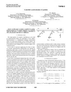
u und v are the image coordinates of the original (distorted) image, ξ and η denote the values of the undistorted image, used in the sequel of this paper. A toolbox [11] previously developed at the institute allows to identify the so defined external and internal camera parameters using different images of a calibration pattern (Fig. 5). These images are taken in each case from a stopped robot (Fig. 4). The poses of the tcp Ta when taking the individual images are assumed to be correctly known. The parameters wi j are then computed by a least-square parameter fit using the Levenberg-Marquardt algorithm [12]. The resulting parameters c Ta are used when computing the kinematics. The internal camera parameters contribute when the undistorted coordinates ξ and η of the detected line points are computed from the image. The determination of the camera parameters cannot be done during the application task since only a calibration object with features distributed over the whole image allows a

Distorted view of the calibration object

consistent parameter estimation. Otherwise a camera model would be built which reproduces the line points correctly only for the test motion. So if no camera calibration as described above is possible a simpler camera model has to be used, e.g. a radial model according to Tsai [13] which as well can represent the barrel distortion of Fig. 5. Svoboda [14] describes a method to determine such a model of lens distortion without using a calibration object. Instead of different images of a single camera, what we would suggest, he uses multiple cameras. B. Execution of a test motion perpendicular to the line After the very camera calibration a purely horizontal translation perpendicular to the line of Fig. 1 is executed. In contrast to the experiment of the next section here we do not use any visual feedback. In this experiment a fixed line point xs is considered for all images. This especially allows to estimate the temporal offset ∆k = kˆ − k (in sampling steps) between the time instant of the exposure kˆ and the internal positional measurement at the robot sampling step k. In addition, scaling errors ∆z are identified. For the chosen motion the camera orientation is constant and aligned with the world system. Then we have ˆ

ˆ

xs = xc(k) + c(k) xˆ s + ∆k · (xc(k+1) − xc(k) ) + ∆z · c(k) xˆ s

∀k. (4) ˆ In contrast to the ideal value c(k) xs of (1) c(k) xˆ s is the sensed position which is computed from the image by the scalar equations of projection

and

ˆ c(k)

ˆ i) · c(k) zs(k+i) xˆs(k+i) = ξ (k,

ˆ

ˆ c(k)

ˆ i) · c(k) zs(k+i) yˆs(k+i) = η(k,

ˆ

ˆ

(5) (6)

using a given distance c(k) zs(k+i) . i is an index of a line point which will be explained in Sect. II-C. Here we only consider i = 0. This is the line point in the center image row of Fig. 2 . If the lines are approximately parallel to the y-axis of the camera system we can replace the vectorial equation

(4) by the scalar equation of the x-component. ˆ

ˆ

xs = xc(k) + c(k) xˆs + ∆k · (xc(k+1) − xc(k) ) + ∆z · c(k) xˆs

∀k, (7)

or ˆ ˆ 0) xs = xc(k) + c(k) zs · ξ (k,

(8)

ˆ ˆ 0) ∀k. +∆k · c(k) xc(k+1) + ∆z · c(k) zs · ξ (k,

The interpolation for the time instant is

The parameters ∆k and ∆z are determined by parameter estimation. The unknown line position is not required if the equation with k = 0 is subtracted in each case. With xc(k) − xc(0) = c(0) xc(k) this yields ˆ

T in homogeneous coordinates instead of the vectorial representations x. Thus (10) is replaced by     ˆ c(k) x xs(l) ˆ s(l) = Tc(k) ˆ · Tα,z · 1 1  ˆ  (11) c(k) x ˆ s(l) c(k) = Tc(k) · Tc(k) ∀k. ˆ · Tα,z · 1

c(k)

ˆ



+∆k · (c(k) xc(k+1) − c(0) xc(1) )

Tα,z =

(9)

ˆ ˆ ˆ 0) − c(0) ˆ 0)) ∀k, +∆z · (c(k) zs · ξ (k, zs · ξ (0,

C. Execution of the application task The third experiment is the application task. This is a feedback controlled following of the online sensed line. In this case a line point xs(l) corresponding to a sampling step l = k + i is visible in the images of multiple time steps k. Parameter estimation is done for each line point by ˆ comparing all positions c(k) xˆ s(l) computed from the images of all time instants kˆ in which the point is visible. With constant orientation of the camera, according to (7) this yields the x-component of the camera system ˆ

ˆ

+∆z · c(k) xˆs(l) − ∆α · c(k) yˆs(l)

∀k.

Rα · (1 + ∆z) 0 0T 1

 (13)

using 

(10) ˆ

∆α is the error in the camera orientation around c(k) z. ˆ and c(k) yˆs(l) are computed using (5) and (6) where ˆ i) and η(k, ˆ i) denote the horizontal and the vertical ξ (k, projective image coordinate of a line point i of the image ˆ The matching between image points taken at time instant k. and line points of a particular sampling step is done using the y-component of the reference trajectory expressed in camera coordinates (see [2]). Equations (10) of different time instants kˆ are compared similar to (9). Like this here in particular the error in the orientation ∆α around the optical axis of the camera system is identified. This is extremely important since for the compensation of time-delays caused by the robot dynamics especially image points at the image border are used for feedforward control. In contrast, for a well suited control, scale errors have only little influence since the line position in the image is almost constant. ˆ c(k) xˆs(l)

The preceding equations are not valid if the orientation of the camera is not constant and aligned with the world system. In that case we have to use transformation matrices

 0 0 . 1

(14)

This yields   xs(l) = Tc(k) · [I + ∆k · (c(k) Tc(k+1) − I)] 1     ˆ (15) c(k) x Rα · (1 + ∆z) 0 ˆ s(l) . · · T 0 1 1   R x Splitting the transformation matrices T = 0T 1 into the rotation matrix R and the translation vector x this yields     Rc(k) xc(k) xs(l) = 1 0T 1    c(k) ( Rc(k+1) − I) c(k) xc(k+1) · I + ∆k · (16) 0T 0     ˆ c(k) x Rα · (1 + ∆z) 0 ˆ s(l) · · 0T 1 1 and finally ˆ

xs(l) = xc(k) + Rc(k) · Rα · (1 + ∆z) · c(k) xˆ s(l) +Rc(k) · ∆k · [c(k) xc(k+1) + (c(k) Rc(k+1) − I) ·Rα · (1 + ∆z) ·

ˆ c(k)

(17)

xˆ s(l) ] ∀k,

where for convenience, we do not use homogeneous coordinates any more. Neglecting products of the small quantities ∆k, ∆z and ∆α yields ˆ

xs(l) = xc(k) + Rc(k) · Rα · c(k) xˆ s(l) ˆ

+Rc(k) · ∆z · c(k) xˆ s(l) + Rc(k) · ∆k · [c(k) xc(k+1) c(k)

D. Application tasks with varying camera orientation

−∆α 1 0

1 Rα =  ∆α 0

where 0ˆ denotes the time instant of the exposure corresponding to time step 0 of the robot.

xs(l) = xc(k) + c(k) xˆs(l) + ∆k · c(k) xc(k+1)

(12)

The matrix Tα,z of the other parameters is set to

ˆ 0) − c(0) zs · ξ (0, ˆ 0) 0 = c(0) xc(k) + c(k) zs · ξ (k,

ˆ

c(k) Tc(k) Tc(k+1) − I). ˆ = I + ∆k · (

+(

Rc(k+1) − I) ·

ˆ c(k)

(18)

xˆ s(l) ] ∀k.

Neglecting changes in the orientation within a single  sampling step c(k) Rc(k+1) − I and inserting (14) yields the x-component

xs(l)

c(l)

= xc(k) ˆ

ˆ ˆ i) + ∆α · ξ (k, ˆ i)) · c(k) +c(l)tc(k),01 · (η(k, zs(l)

ˆ

+ tc(k),00 · (c(k) xˆs(l) − ∆α · c(k) yˆs(l)

ˆ

ˆ

+c(l)tc(k),02 · c(k) zs(l)

+∆z · c(k) xˆs(l) + ∆k · c(k) xc(k+1) ) ˆ

ˆ

+ tc(k),01 · (c(k) yˆs(l) + ∆α · c(k) xˆs(l) +∆z · ˆ c(k)

+ tc(k),02 · (

ˆ c(k)

yˆs(l) + ∆k · c(k) yc(k+1) )

zˆs(l) ˆ

where tc(k),i1 i2 denotes the element i1 , i2 of the transformation matrix Tc(k) . For Rc(k) = I, equation (19) is identical to (10). Now we express (19) in the camera system of time step l. Inserting (5) and (6) and subtracting the equation of k = l, i.e. the equation with i = 0 and kˆ = l,ˆ yields xc(k)

h ˆ ˆ i) − ∆α · η(k, ˆ i)) · c(k) +c(l)tc(k),00 · ((1 + ∆z) · ξ (k, zs(l) i +∆k · c(k) xc(k+1) h ˆ ˆ i) + ∆α · ξ (k, ˆ i)) · c(k) +c(l)tc(k),01 · ((1 + ∆z) · η(k, zs(l) i (20) +∆k · c(k) yc(k+1) ˆ

+c(l)tc(k),02 · [(1 + ∆z) · c(k) zs(l) + ∆k · c(k) zc(k+1) ] ˆ 0) − ∆α · η(l, ˆ 0)) · c(l)ˆ zs(l) = ((1 + ∆z) · ξ (l, +∆k · c(l) xc(l+1)

ˆ

ˆ 0) − ∆α · η(l, ˆ 0)) · c(l) zs(l) = (ξ (l,

(19)

+∆z · c(k) zˆs(l) + ∆k · c(k) zc(k+1) ) ∀k,

c(l)

ˆ ˆ i) − ∆α · η(k, ˆ i)) · c(k) xc(k) + c(l)tc(k),00 · (ξ (k, zs(l)

∀k.

We propose to determine ∆k and ∆z according to Sect. IIB since at least ∆z cannot be determined with a small control error. Then, here we can restrict on the estimation of ∆α. After convergence we try to improve the result by refining ∆k as well. The estimated parameters can be applied in the camera module for the interpolation of the time instant of the exposure and for the mapping. Then here in the estimation module the remaining calibration errors will be ∆z = 0 und ∆k = 0. In this case we get ∆α without the above mentioned approximations using

(21)

∀k.

Since c(k) ys(l) and c(k) zs(l) are given for each time step l ˆ by the reference trajectory, we can interpolate c(k) ys(l) and ˆ c(k) z ˆ s(l) . Equation (6) then allows to compute η(k, i) which ˆ has to be given to get ξ (k, i) from the image. Thus each equation of a line point which is visible at time kˆ and lˆ yields a value for ∆α. These values have to be filtered to get the result. III. E XPERIMENTAL R ESULTS The method is demonstrated using the cable tracking experiment of Sect. I. By compensation of the errors in the way explained in Sect. II the system is improved: With a well calibrated camera the mean path error is about 50 % of that of the experiment without calibration. Once again a reduction of almost 50 % is reached when adapting the other parameters by some runs using (9) and further runs with (21) thereafter. The results are listed in Table I and Figures 6 and 7, including experiments with a reduced number of adapted parameters. Run #7 would yield similar results with (20) and without (9), but then the adaptation would need about 10 runs to converge. Table I demonstrates that for our scenario the estimation of the scale ∆z and of the external camera parameters c Ta may be omitted. The importance of the scale depends on the desired distance of the line from the image center. Important errors in the external camera parameters are compensated by other parameters. In contrast, without knowing the internal camera parameters wi j no satisfying control is possible. The parameter errors detected in the experiment are 0.010 s time offset, 0.005 rad orientational error, and TABLE I R EMAINING MEAN PATH DEVIATIONS WHEN FOLLOWING A CURVED LINE . (T HE ERRORS ARE COMPUTED FROM THE CENTER IMAGE ROW. T HE MAXIMUM OBSERVED ERRORS DURING THE EXPERIMENT ARE DISPLAYED IN BRACKETS .

T HE LOWER THREE ROWS CORRESPOND TO

A CHANGED LAYOUT OF THE LINE USING THE PREVIOUSLY ADAPTED PARAMETERS )

Fig. 6. Improvement by camera calibration when following a curved line: The solid blue line corresponds to #1 of table I, the dashed red line to #2

1 2 3 4 5 6 7 8 11 12 13

compensation of errors in cT wi j ∆k ∆α ∆z a + + + + + + + + + + + + + + + + + + + + + + + + + + + + + + + + +

image error (pixel) 2.31 (4.2) 1.05 (2.8) 2.20 (4.8) 0.52 (1.5) 0.96 (2.0) 0.67 (2.5) 0.53 (1.8) 0.51 (1.9) 1.95 (4.1) 1.40 (3.6) 0.47 (1.3)

path error (mm) 0.99 (1.8) 0.53 (1.5) 0.95 (2.1) 0.20 (0.5) 0.48 (1.2) 0.39 (1.4) 0.33 (1.1) 0.32 (1.1) 0.84 (1.8) 0.64 (2.0) 0.26 (0.7)

Fig. 7. Improvement by adaptation of the other parameters: The dashed red line corresponds to #12 of table I, the solid blue line to #13

10 mm distance error. These values are then used with a totally different layout of the line. This proves the portability of the adapted parameters (see lower part of Table I and Figures 7 and 8). IV. C ONCLUSION We have developed a method that enables a robot manipulator to follow lines that are visible by a robot mounted camera. For high speed motion the parameters of the camera and of the interaction between robot and camera have been identified. In contrast to the tracking of moving objects as described by [15], [16] the accuracy can be very high when following motionless edges since in this case there are no future accelerations of the target that could affect the performance. High performance, however, can only be reached if the vision system and the controller are tuned and synchronized. This has be done using the application task, thus yielding unbiased parameters. The experiments documented in Sect. III do not show the calibration error directly. Instead they are the result from the cooperation of camera, vision algorithms, control, and the robot dynamics when executing a fast motion (0.7 m/s speed along the path) with huge a priori uncertainties (see Fig. 8). To the knowledge of the authors no other approach reaches such an accuracy at this speed. The achieved mean pixel error of half a pixel will certainly only be outperformed with high costs. For further increase of the accuracy a high resolution camera will be required that combines precision in the horizontal image component (line position) with a wide

Fig. 8. Sensed path correction with respect to the reference path (The dashed red line corresponds to #13 of table I, the solid blue line to #8

range in the vertical component (prediction of the line points of future time steps). Besides, the robot hardware has to be improved. Alternatively an external measuring device might be used to survey the camera position. Otherwise joint elasticity which is present also with industrial robots, will limit the accuracy, as can be seen by (1). Previous approaches [17] for compensation of joint elasticities when using the architecture of Fig. 3 propose external measuring devices for both adaptation of the ideal robot and determination of the real arm trajectory. In contrast static deviations of the robot position caused by elasticity only play a minor role for fast sensor based motion. The same is true if the kinematic parameters are only roughly known. R EFERENCES [1] F. Lange and G. Hirzinger. A universal sensor control architecture considering robot dynamics. In Proc. Int. Conf. on Multisensor Fusion and Integration for Intelligent Systems, pages 277–282, Baden-Baden, Germany, August 2001. [2] F. Lange and G. Hirzinger. Spatial control of high speed robot arms using a tilted camera. In Int. Symposium on Robotics (ISR 2004), Paris, France, March 2004. [3] F. Lange and G. Hirzinger. Learning of a controller for non-recurring fast movements. Advanced Robotics, 10(2):229–244, April 1996. [4] M. Grotjahn and B. Heimann. Model-based feedforward control in industrial robotics. The International Journal on Robotics Research, 21(1):45–60, January 2002. [5] J. A. Gangloff and M. F. de Mathelin. Visual servoing of a 6-dof manipulator for unknown 3-d profile following. IEEE Trans. on Robotics and Automation, 18(4):511–520, August 2002. [6] D. Caltabiano, G. Muscato, and F. Russo. Localization and self calibration of a robot for volcano exploration. In Proc. 2004 IEEE Int. Conf. on Robotics and Automation (ICRA), pages 586–591, New Orleans, LA, April 2004. [7] Y. Liu et al. A new generic model for vision based tracking in robotic systems. In Proc. 2003 IEEE/RSJ Int. Conf. on Intelligent Robots and Systems (IROS), pages 248–253, Las Vegas, Nevada, Oct. 2003. [8] V. Kyrki, D. Kragic, and H. I. Christensen. Measurement errors in visual servoing. In Proc. 2004 IEEE Int. Conf. on Robotics and Automation (ICRA), pages 1861–1867, New Orleans, LA, April 2004. [9] J.-M. Frahm and R. Koch. Robust camera calibration from images and rotation data. In 25th Pattern Recognition Symposium, DAGM’03, Magdeburg, Germany, Sept. 2003. Springer-Verlag, Heidelberg. [10] J. Weng, P. Cohen, and M. Herniou. Camera calibration with distortion models and accuracy analysis. IEEE Trans. on Pattern Analysis and Machine Intelligence, 14(10):965–980, Oct. 1992. [11] http://www.robotic.dlr.de/vision/projects/Calibration/, 2004. [12] W. H. Press, B. P. Flannery, S. A. Teukolsky, and W. T. Vetterling. Numerical Recipes in C. Cambridge University Press, 1988. [13] R. Y. Tsai and R. K. Lenz. A new technique for fully autonomous and efficient 3D robotics hand/eye calibration. IEEE Trans. Robotics and Automation, 5(3):345–358, 1989. [14] Tom´as˘ Svoboda. Quick guide to multi-camera self-calibration. Technical Report BiWi-TR-263, Computer Vision Lab, Swiss Federal Institute of Technology, Z¨urich, Switzerland, August 2003. http://cmp.felk.cvut.cz/˜svoboda/SelfCal/Publ/ selfcal.pdf. [15] S. Hutchinson, G. D. Hager, and P. I. Corke. A tutorial on visual servo control. IEEE Trans. on Robotics and Automation, 12(5):651– 670, Oct. 1996. [16] A. Namiki, K. Hashimoto, and M. Ishikawa. A hierarchical control architecture for high-speed visual servoing. The International Journal on Robotics Research, 22(10-11):873–888, Oct-Nov 2003. [17] F. Lange and G. Hirzinger. Learning accurate path control of industrial robots with joint elasticity. In Proc. IEEE Int. Conference on Robotics and Automation, pages 2084–2089, Detroit, Michigan, May 1999.