magnetically disturbed environment onboard a jet aircraft. I. INTRODUCTION .... also be taken when entering or leaving buildings or rooms during calibration.
Calibration of a magnetometer in combination with inertial sensors Manon Kok∗ , Jeroen D. Hol† , Thomas B. Sch¨on∗ , Fredrik Gustafsson∗ and Henk Luinge† ∗ Division
of Automatic Control Link¨oping University, Sweden Email: {manon.kok, thomas.schon, fredrik.gustafsson}@liu.se † Xsens Technologies B.V. Enschede, the Netherlands Email: {jeroen.hol, henk.luinge}@xsens.com
Abstract—Measurements from magnetometers and inertial sensors (accelerometers and gyroscopes) can be combined to give 3D orientation estimates. In order to obtain accurate orientation estimates it is imperative that the magnetometer and inertial sensor axes are aligned and that the magnetometer is properly calibrated for both sensor errors as well as presence of magnetic distortions. In this work we derive an easy-to-use calibration algorithm that can be used to calibrate a combination of a magnetometer and inertial sensors. The algorithm compensates for any static magnetic distortions created by the sensor platform, magnetometer sensor errors and determines the alignment between the magnetometer and the inertial sensor axes. The resulting calibration procedure does not require any additional hardware. We make use of probabilistic models and obtain the calibration algorithm as the solution to a maximum likelihood problem. The efficacy of the proposed algorithm is illustrated using experimental data collected from a sensor unit placed in a magnetically disturbed environment onboard a jet aircraft.
I. I NTRODUCTION Accelerometers and gyroscopes (inertial sensors) in combination with magnetometers are generally available in standalone sensor units, but also in devices such as mobile phones and aircraft. To estimate orientation from these sensor measurements extended Kalman filters (EKFs) can be used. Accelerometer measurements can be used to observe inclination in the case that the linear acceleration of the body is much smaller then the earth gravity vector. The rotation around the earth gravity vector cannot be observed from accelerometer measurements. The angle with respect to the magnetic north, referred to as heading, can be observed using magnetometers. In a magnetically undisturbed environment, magnetometers measure the local earth magnetic field consisting of a vertical component and a horizontal component pointing in the direction of the magnetic north. A combination of magnetometers and inertial sensors can therefore be used to estimate 3D orientation. For this purpose, however, it is imperative that the sensor axes of the inertial sensors and the magnetometer are aligned. In the absence of magnetic field distortions, a magnetometer is a reliable source of information due to its high sampling rate and reliable sensor readings. In the presence of magnetic field disturbances, however, erroneous heading estimates will be obtained since the magnetometer no longer measures only
1
1
0
0
−1
−1 −1
−1
0 −1
0
1
1
(a) Original measurements
0 −1
0
1
1
(b) Calibrated measurements
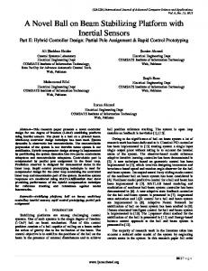
Fig. 1. Results from the Delphin flight test discussed in Section VI-B. As shown, a calibration of the ellipsoid of data {y m,k }K k=1 leads to calibrated measurements lying on the unit sphere.
the earth magnetic field. This problem occurs for instance when mounting the magnetometer in a car, an aircraft or a mobile phone and re-calibration is needed each time the magnetic disturbance changes. It is therefore important to always calibrate the magnetometer before use. The aim of this paper is to derive a magnetometer calibration algorithm which will account for 1) magnetometer sensor errors, 2) presence of magnetic disturbances caused by mounting of the magnetometer, 3) misalignment between magnetometer and inertial sensor axes. Existing approaches [1]–[6] have focussed on stand-alone magnetometer calibration and have therefore only considered item 1 and 2 in the list above. However, when magnetometers are used in combination with inertial sensors, item 3 becomes crucial to obtain good orientation estimates. To perform the suggested calibration, the magnetometer and inertial sensors need to be rigidly mounted on the platform to be used, for instance a mobile phone, an aircraft or a car. Data subsequently needs to be collected while rotating the platform in all possible orientations. For a properly calibrated magnetometer the magnitude of the measured magnetic field is not dependent on the orientation of the platform, implying that the collected magnetometer data lies on a sphere. The presence of magnetic distortions and/or magnetometer sensor
errors will cause the magnetometer data to lie on an ellipsoid instead. Accounting for these errors will therefore map the ellipsoid of magnetometer data to a sphere, where we without loss of generality assume that this is the unit sphere. In Figure 1 an illustration of the ellipsoid of experimental data and the calibration results can be found. For stand-alone magnetometers the mapping of the ellipsoid of data to a sphere gives a complete magnetometer calibration. However, combining the magnetometer with inertial sensors requires the sensor axes to be aligned, i.e. the sphere needs to be rotated such that the magnetometer sensor axes are aligned with the inertial sensor axes. The complete calibration problem is posed and solved as a maximum likelihood (ML) problem. Since this is a non-convex optimization problem, a three-step procedure is described to obtain a good initial estimate for the ML calibration problem. Experimental results will be discussed in Section VI and will show that the calibrated data lies on a unit sphere, as shown in Figure 1, and is aligned with the inertial sensor axes. II. M ODEL To be able to formulate the calibration problem as a maximum likelihood problem, a proper model of the magnetometer measurements is needed. Here, both the magnetometer data itself as well as the relation between the rotation of the sphere and the inertial measurements needs to be modeled. A. Magnetometer measurement model A model of the magnetometer measurements relates the measurement data set {y bm,k }K k=1 to the local magnetic field mn . Here b denotes the body frame of the magnetometer, n denotes the navigation frame and k denotes the sample number. The rotation of sample k from navigation frame n to body frame b will be defined as Rkbn . Defining the local magnetic field in body frame, mbk , as mbk = Rkbn mn , {y bm,k }K k=1
{mbk }K k=1 .
(1)
we would hope for = However, there are two reasons why they will in practice generally not be equal and calibration is needed. 1) Sensor errors in the magnetometer triad: A first source of error is sensor errors, which are sensor-specific and can differ for each magnetometer triad. These sensor errors consist of four components [1], [4], [5]. 1) Non-orthogonality of the magnetometer axes. We will define the 3 × 3 matrix Cno representing this nonorthogonality. 2) Presence of a zero bias or null shift, implying that the magnetometer will measure a non-zero magnetic field even if the magnetic field is zero, defined by ozb . 3) Difference in sensitivity of the three magnetometer axes, represented by a diagonal 3 × 3 matrix Csc . 4) Presence of noise in the magnetometer measurements. We will assume this noise to be independently and identically distributed (i.i.d.) Gaussian noise and it will be denoted by ebm .
This leads to the following relationship between mbk and y bm,k , accounting only for the sensor errors y bm,k = Csc Cno mbk + ozb + ebm,k .
(2)
2) Presence of magnetic disturbances: In the vicinity of magnetic materials, a magnetometer will not only measure the local magnetic field, but also an additional magnetic field component. We assume that all magnetic disturbances present are stationary and constant, i.e. rigidly attached to the sensor, for instance due to mounting of the magnetometer in a phone, a car or an aircraft. Calibration of temporary or time-varying magnetic disturbances is very challenging and will not be considered in this paper. Ferromagnetic materials can lead to both so-called hard and soft iron effects. Hard iron effects are due to the permanent magnetization of the magnetic material and lead to a constant additional magnetic field. The vector representing these effects is denoted as ohi . Soft iron effects are due to magnetization of the material as a result of an external magnetic field and will therefore depend on the orientation of the material with respect to the external field. It can change both the magnitude and the orientation of the measured magnetic field. The 3 × 3 matrix representing the soft iron effect is denoted as Csi . Given the correct mapping parameters, one is able to completely calibrate for the hard and soft iron effects. After applying the calibration the magnetometer measurements will represent the field as if there were no magnetic distortions due to the ferromagnetic object. Note that in accordance to existing literature we assume a linear relation between the field that the soft iron generates and the external magnetic field, i.e. we assume that no hysteresis occurs. As argued in [1] this is a reasonable assumption since hysteresis will only occur when very large magnetic fields are applied. Extending (2) to also include the model of the magnetic disturbances introduced above, results in y bm,k = Csc Cno (Csi mbk + ohi ) + ozb + ebm,k .
(3)
3) Magnetometer model assumptions: For the model (3) to be valid the following two requirements need to be satisfied: • All present magnetic distortions need to be constant and stationary, i.e. rigidly attached to the sensor, for instance due to mounting of the magnetometer in a phone, a car or an aircraft. n • The local magnetic field mk will be assumed constant, i.e. to be equal for all samples k. This is a physically reasonable assumption as long as the distance travelled during calibration is not of the order of parts of the earth. However, care should also be taken when entering or leaving buildings or rooms during calibration. Assuming that the requirements are satisfied, (1) implies that the local magnetic field in body frame mbk will lie on a sphere with a radius equal to the magnitude of the local magnetic field. From (3) we therefore expect the data y bm,k to lie on an ellipsoid which can be translated, rotated, skewed and scaled with respect to this sphere. The number and spread of
measurements over the ellipsoid depends on the orientations of the magnetometer during the measurement collection for calibration. Previous work has used similar magnetometer measurement models as (3) [1]–[6]. Using these methods, the rotation of the resulting magnetometer calibration is still ambiguous up to a fixed rotation. This paper will therefore extend existing approaches and fix the orientation of the sphere based on the inclusion of inertial measurements. The existing magnetometer measurement model will first be extended to include the rotation between the inertial and magnetometer sensor axes. Subsequently, the rotation of the sphere will be modeled. 4) Magnetometer and inertial sensor axes alignment: Extending (3) with a rotation matrix Rim describing the misalignment between the inertial sensors and the magnetometer results in y bm,k = Csc Cno (Csi Rim mbk + ohi ) + ozb + ebm,k .
(4)
5) Resulting calibration model: To obtain a correct calibration, it is not necessary to identify all individual contributions of the different components in (4). Instead, they can be combined into a 3 × 3 distortion matrix D and a 3 × 1 offset vector o where D = Csc Cno Csi Rim ,
(5a)
o = Csc Cno ohi + ozb ,
(5b)
leading to the resulting magnetometer measurement model y bm,k = Dmbk + o + ebm,k .
(6)
B. Rotation of the sphere As discussed in the previous section, magnetometer data can be compensated for sensor errors and the presence of magnetic distortions by mapping an ellipsoid of data to a sphere. The rotation of the sphere can, however, not be determined from magnetometer measurements only. Determining this rotation is important when combining magnetometer measurements with inertial measurements, for instance for orientation estimation. The rotation of the sphere can be determined by using both the magnetometer measurements and processed measurements of the vertical {y z,k }K k=1 , defined by y bz,k = Rkbn z n + ebz,k ,
(7)
� �T where z n = 0 0 1 . The noise ebz,k is assumed to be Gaussian. The processed measurements {y z,k }K k=1 can for instance be obtained by keeping the accelerometer stationary in different orientations. In that case, only the gravity vector is measured, indicating the direction of the vertical. Alternatively, the vertical measurements can be obtained by running an extended Kalman filter estimating inclination based on inertial measurements. As discussed in Section I, the local earth magnetic field mn will consist of a horizontal component pointing in the direction
mn
d
δ
Fig. 2. Schematic of a part of the earth where the earth magnetic field mn makes an angle δ with the horizontal plane. The vertical component of mn defined by mn sin δ, will be denoted by d.
of the magnetic north and a vertical component, �p �T mn = ||mn ||22 − d2 0 d � �T = ||mn ||2 cos δ 0 − sin δ ,
(8)
where δ denotes the dip angle, the angle between mn and the horizontal plane, and d is the vertical component of mn as depicted in Figure 2. Inclusion of the magnetic declination, the angle between true and magnetic north, in (8) would lead to a non-zero second component of mn . Since the calibration results D and o in (6) only depend on the ratio between the horizontal and vertical components, we can without loss of generality assume that mny is zero. Both the norm of mn and the dip angle δ are assumed to be constant. They depend on the location on the earth but can deviate from that in indoor or otherwise magnetically disturbed environments. Since our algorithm does not use any prior knowledge on the dip angle or the strength of the magnetic field it also works in indoor or otherwise homogeneously magnetically disturbed environments. As can be seen from (8) and the definition of z n , the inner product of mn and z n is equal to d. The inner product of Rkbn mn and Rkbn z n is therefore also equal to d for all possible rotations Rkbn . When the inertial and magnetometer sensor axes are not aligned, however, the estimated d based on the magnetometer and vertical measurements will differ for each Rkbn , as schematically depicted in Figure 3. The rotation of the sphere is chosen such that the inertial and magnetometer sensor axes are aligned and the estimated dip angle d becomes approximately constant. For the model of the rotation of the sphere to be accurate, • the dip angle needs to be constant for all measurements k and • the relation between the inertial and the magnetometer sensor axes needs to be described by a rotation matrix only, i.e. we assume that no mirroring of axes takes place. The first requirement is again a physically reasonable assumption as long as the distance travelled during calibration is not of the order of parts of the earth, similar to the requirement discussed in Section II-A3. The second requirement can easily be satisfied by proper mounting of the sensor axes. In the remainder we implicitly assume all measurements y and noises e to be in the body frame, dropping the superscript b.
zn
We will find an estimate of the unknown parameters θ 1 , θ 2 by solving the associated maximum likelihood problem bML = arg max p (y ), θ 1:k θ
(13)
θ 1 ,θ 2
where y 1:k , {y m,1 , y z,1 , . . . , y m,k , y z,k }. Assuming independent Gaussian noise reduces the ML problem to
d0 d
K
n m n
m0
θ 1 ,θ 2
Fig. 3. The vertical component of the local earth magnetic field d can also be defined as the inner product of the vectors mn and z n . In case the magnetometer sensor axes are rotated with respect to the inertial sensor axes leading to a measurement m0 n , the resulting vertical component d0 differs from d.
III. M AXIMUM LIKELIHOOD FORMULATION In Section II-A a model was derived for the magnetometer measurements as a function of the local magnetic field, the distortion matrix D and the offset vector o. As argued, we expect the measurements to lie on an ellipsoid before calibration and to lie on a sphere with radius ||mn ||2 after calibration. The magnitude of the magnetometer readings is irrelevant in most applications, for instance in the case of orientation estimation. The radius of the sphere will in this paper without loss of generality be scaled to one, i.e. ||mn ||2 = 1. However, other options like scaling towards the magnitude of the local magnetic field in Gauss or Tesla are of course also possible. In Section II-B a model relating the inertial and magnetometer measurements to determine the rotation of the sphere of magnetometer data was introduced. The models from Sections II-A and II-B will be combined and used in a maximum likelihood (ML) problem. Combining (6) and (1) results in y m,k = DRkbn mn + o + em,k ,
(9a)
where from Section II we know that mn is constant and given by (8). Furthermore, the measurements of the vertical are defined by (7), which for clarity is repeated here, y z,k = Rkbn z n + ez,k .
(9b)
We define the parameter θ 1 as θ 1 = {D, o, mn , {Rkbn }K k=1 }, D∈R n
3×3 3
m ∈ {R : {Rkbn }K k=1
3
o∈R ,
,
||mn ||22
� 1 X� ||em,k ||2Σ−1 + ||ez,k ||2Σ−1 m z 2
bML = arg min θ
=
1, mny
(10)
where mny denotes the second component of the vector mn . Assuming the noise to be independent and Gaussian, em,k ∼ N (0, Σm ),
(11a)
ez,k ∼ N (0, Σz ),
(11b)
IV. C OMPUTING AN INITIAL ESTIMATE n b 0, o bbn }K } b0 , m c0 , {R To obtain a good initial estimate {D 0,k k=1 for the ML problem (14), a three-step algorithm is used. The first step maps the magnetometer data to a unit sphere b0 and can partially determine and obtains initial estimates o b 0 , where the estimate after the ellipse fit is denoted D e 0. A D second step determines the rotation between the inertial and n b 0 and m c0 . magnetometer measurements to obtain estimates D A third step uses the results from the previous steps to obtain bbn }K . estimates of the rotations {R 0,k k=1 A. Ellipse fit As a first step, we focus on the magnetic field measurements. As mentioned in the previous section, we scale the norm of the local magnetic field such that ||mn ||2 = 1. This leads to 0 = ||mn ||22 − 1 = ||Rknb mbk ||22 − 1 = ||mbk ||22 − 1 ≈ y Tm,k Ay m,k + bT y m,k + c,
Σm ∈ {R3x3 : Σm = ΣTm , Σm � 0}, (12)
(15)
where the noise em,k is neglected and we introduced the notation A , D−T D−1 , T
T
b , −2o D T
c,o D
we define the parameter θ 2 as θ 2 = {Σm , Σz }, Σz ∈ {R3x3 : Σz = ΣTz , Σz � 0}.
K K log det Σm + log det Σz . (14) 2 2 The requirements on θ 1 in (10) do not need to enter as constraints in the optimization problem, when parametrizing the rotation matrices with three components and mn with one component. In Section VI we have assumed Σm and Σz to be diagonal. The results are obtained by first solving for θ 1 assuming θ 2 to be identity, afterwards solving for θ 2 given θ 1 and subsequently solving for θ 1 given the obtained θ 2 instead of solving the complete problem (14) at once. The ML problem (14) is a non-convex optimization problem requiring a good initial estimate for θ 1 . This initial estimate is obtained by a three-step algorithm described in the subsequent section. +
= ||D−1 (y m,k − o − em,k )||22 − 1
= 0},
∈ SO(3),
k=1
−T
−T
D
(16a) D
−1
−1
,
(16b)
o − 1.
(16c)
This can be recognized as the definition of an ellipsoid. A standard ellipse fitting approach can be taken to determine A, b and c. We use the least squares approach introduced in
[7]. As argued by [5], an adaptive least squares approach as described in [8] leads to better, unbiased estimates. However, since our approach uses the ellipse fitting only as an initial estimate for the final ML problem, a least squares approach is sufficient. It is straightforward to rewrite (15) as a linear relation in η according to Jη ≈ 0,
(17)
e 0 , obtained by Cholesky Denoting a solution to (23a) by D decomposition, the eventual solution can there be defined as b0 = D e 0 R, D
(24)
where the unknown rotation matrix R will be determined in Section IV-B. Supporting data is needed to determine the rotation matrix R. For this, measurements of the vertical will be used. B. Determine the rotation of the ellipse
with � J = y Tm,k ⊗ y Tm,k vecA η = b , c
y Tm,k
� 1 ,
(18a) (18b)
where ⊗ denotes the Kronecker product and vec denotes the vectorization operator. This problem can be solved by assuming that the matrix A is symmetric. An easy way to obtain a solution is through a b singular value decomposition of the matrix J. The solution η is the right eigenvector corresponding to the smallest singular value of J [7]. Obtaining the solution in this way automatically avoids the trivial zero solution since the norm of the obtained b is by definition equal to 1. solution vector η Since any αη will be an equally valid solution to (17), we will only find a scaled version of our desired solution. Defining the obtained solution as bs vecA b= b η (19) bs , b cs and the desired solution as b vecA b η, b = αb
(20)
b c the scaling factor α can be determined from (16)
In Section IV-A the measurements were fitted to an ellipse, but the rotation R in (24) is still unknown. A second step in obtaining the initial estimate θ 0 is to determine this rotation matrix R. As discussed in II-B and illustrated in Figure 3, this can be done by imposing the assumption that the vertical component of the estimated local magnetic field should be constant for all k, resulting in the following optimization problem min R,d
s.t.
(25)
C. Initial estimate of {Rkbn }K k=1 From Sections IV-A and IV-B we have obtained initial n b 0, o b0 and m c0 . These can be used in combination estimates D with (1), (7) to obtain initial estimates for {Rkbn }K k=1 . Applying Theorem 4.1 in [9], the rotation quaternion qkbn is given by the eigenvector corresponding to the largest eigenvalue of Ak , b
= 14 bT A−1 b − c =
k=1
R ∈ SO(3),
The optimization can be initialized with R = I3 and d = 0. b in (25), an initial estimate D b 0 can be From the estimated R b obtained using (24). The estimate d can be used to obtain an n c0 according to initial estimate of m hp iT n c0 = m (26) 1 − db2 0 db .
1 = oT D−T D−1 o − c α( 14 bTs A−1 s bs
K � 1X e −1 y m,k − o ||22 ||d − y Tz,k RT D 0 2
Ak = −(c m0,k )L (c m0 )R − (y bz,k )L (z n )R ,
n
(27)
� b b −1 y m,k − o c0 = D b0 , m 0
(28)
where
− cs ),
(21)
leading to
and α=
�
1 T −1 4 b s As b s
− cs
�−1
.
(22)
This ellipse fitting step is a first step towards obtaining the e 0 and initial estimate θ 0 and its components will be denoted D b0 , where from (16) o b −T D b −1 D 0 0
bs , = αA b b−1 b0 = − 12 A o s bs .
(23a) (23b)
b 0 . Any From (23a) it is not possible to uniquely determine D b 0 U where U U T = I3 will also fulfill (23a). As described D in Section II-B, we assume that the sensor axes of the inertial sensors and the magnetometers are only related by a rotation.
0 y x yL = yy yz 0 yx R y = yy yz
−yx 0 yz −yy
−yy −yz 0 yx
−yx 0 −yz yy
−yy yz 0 −yx
−yz yy , −yx 0 −yz −yy . yx 0
(29a)
(29b)
Here, yx , yy , yz denote the first, the second and the third components of y respectively. bbn }K can be obtained by straightforInitial estimates {R 0,k k=1 ward conversion of the quaternions {qkbn }K k=1 .
V. C OMPLETE ALGORITHM
−0.4
The complete algorithm is summarized in Algorithm 1. The algorithm requires magnetometer measurements and processed vertical measurements, where the latter can be obtained from inertial measurements as described in Section II-B. Collect b K data {y bm,k }K k=1 and {y z,k }k=1 by rotating the assembly in all possible orientations, so that the magnetometer measurements describe (a part of) an ellipsoid. During collection of the measurements, the inertial sensors and magnetometer need to be rigidly attached to each other. Furthermore, they need to be rigidly mounted onto the platform, for instance a phone or an aircraft. Make sure that the calibration takes place in an otherwise homogeneous magnetic field. Also avoid proximity of objects generating non-constant magnetic fields.
−0.5
Algorithm 1 Magnetometer and inertial calibration n b 0, o bbn }K b0 , m c0 and {R 1) Obtain initial estimates D 0,k k=1 a) Perform an ellipse fit as described in Section IV-A e 0 and o b0 . to obtain D b) Determine the rotation of the ellipse as described n b 0 and m c0 . in Section IV-B to obtain D bn K b c) Determine the rotations {R0,k }k=1 as described in Section IV-C. 2) Compute the ML estimate using (14), starting the opn b0 = {D bbn }K , I3 , I3 } to b 0, o b0 , m c0 , {R timization in θ 0,k k=1 n bn K b b b b m, Σ b z }. b, m c , {Rk }k=1 , Σ obtain θ ML = {D, o b and o b to the magnetometer data in 3) Apply the obtained D subsequent measurements to obtain measurements that are calibrated for the relevant setup.
ym yv m yv
−0.6
d
−0.7 −0.8 −0.9 −1 −1.1 0
50
100
150
200 250 Sample [#]
300
350
400
Fig. 4. The vertical component of mn (d, see Figure 2 for definition) for the experiment discussed in Section VI, estimated from data before (grey dashed line) and after calibration (black solid line). 300
350 300
250
250 200 200 150 150 100 100 50
0 −5
50
0
5
0 −5
0
5
Fig. 5. Residuals of ML problem for the experiment discussed in Section VI. Left: Residuals related to (9a); Right: Residuals related to (9b).
VI. E XPERIMENTAL RESULTS In this section, calibration results from two experiments will be presented. The first experiment is performed to test the calibration results for a misalignment between the inertial sensors and the magnetometer. The second experiment shows calibration results for a sensor mounted in a magnetically disturbed environment onboard a jet aircraft. It shows that the calibration algorithm works well for real-world applications, also with limited rotation possibility. A. Misalignment magnetometer inertial sensor axes Algorithm 1 has been used to correct for a possible misalignment between the accelerometer and magnetometer sensor axes. Data has been collected with a standalone sensor unit with aligned magnetometer and accelerometer axes, from which the accelerometer data has been rotated by 30 degrees around the y-axis. The vertical measurements are obtained by keeping the sensor unit stationary in different orientations. Since a calibration using the same algorithm is performed before rotating the data, the expected calibration results only show a rotation of the sensor axes.
The obtained calibration results are 2.4 3.5 0.86 −0.00 −0.50 b = −0.01 1.01 −0.00 ± 6.8 2.5 D 2.3 4.1 0.50 0.00 0.87 7.3 1.5 b = − 0.3 10−3 ± 2.9 10−3 . o 0.6 1.0
1.9 3.0 10−3 , 1.5 (30)
As expected, these show only a rotation around the y-axis of −30 degrees, which compensates the applied rotation of the accelerometer measurements. As described in Section II-B the inner product of the local magnetic field and the vertical measurements gives the vertical component of mn , defined as d according to (8). When the misalignment between the magnetometer and the inertial sensor axes has been properly calibrated for, the estimated d is constant for all rotations. In Figure 4 the vertical component of the estimated local magnetic field, before and after calibration is shown. As can be seen, d is much more constant after calibration. The residuals from the ML problem are depicted in Figure 5, showing that the problem gives reasonable residuals.
in a nonlinear optimization problem. In order to obtain a good solution to this problem we are relying on a good initialization, which is provided by a three-step approach. The real world experiments illustrate that the algorithm appears to perform well and that it is indeed capable of correcting for both magnetic field distortions and misalignment between the inertial and the magnetometer sensor axes. ACKNOWLEDGMENT This work is supported by MC Impulse, a European Commission, FP7 research project and CADICS, a Linnaeus Center funded by the Swedish Research Council (VR). Fig. 6. The Aero L-29 Delphin jet aircraft used for the experiments reported in Section VI-B.
B. Delphin flight test A second experiment has been performed by collecting data from inertial sensors and a magnetometer in an Aero L-29 Delphin jet aircraft shown in Figure 6 [9]. The inertial sensors and the magnetometer are in this case aligned, but the magnetometer suffers from magnetic distortions due to its mounting in the metallic aircraft. Since the aircraft experiences high accelerations, the accelerometer measurements are not a good source of vertical measurements in this case. The vertical measurements {y z,k }K k=1 are instead obtained using an EKF estimating the aircraft’s inclination based on inertial measurements. The aircraft is not able to easily rotate into all orientations, but some looping maneuvers were performed. As shown in Figure 1 the calibration results lie on a unit sphere even if not all rotations are present. The obtained calibration results including their 99% confidence intervals are 1.6 1.1 1.2 0.86 −0.02 0.08 b = −0.04 0.94 −0.16 ± 1.6 0.7 0.8 10−2 , D 1.5 0.9 0.5 0.15 0.03 1.22 7.6 −0.14 b = − 0.06 ± 4.5 10−3 . (31) o 5.0 0.10 b and offset vector o b show The determined distortion matrix D a significant correction for magnetic field distortions, as visualized in Figure 1. Correcting for these magnetic distortions will lead to a significant improvement of the heading estimate. In Section 8.2.2 in [9], the calibrated magnetometer data is used in an EKF together with inertial and GPS measurements to obtain orientation and position estimates, where applying Algorithm 1 to the magnetometer data improves the root mean square error (RMSE) in the heading from 43.2 to 1.8 degrees. VII. C ONCLUSION A magnetometer calibration algorithm has been developed, capable of both determining the misalignment between the inertial sensors and the magnetometer as well as compensating for magnetometer sensor errors and magnetic distortions arising from the sensor platform. The calibration algorithm was derived using a maximum likelihood formulation resulting
R EFERENCES [1] D. Gebre-Egziabher, G. H. Elkaim, J. D. Powell, and B. W. Parkinson, “Calibration of strapdown magnetometers in magnetic field domain,” Journal of Aerospace Engineering, pp. 87–102, Apr. 2006. [2] R. Alonso and M. D. Shuster, “Complete linear attitude-independent magnetometer calibration,” The Journal of the Astronautical Sciences, vol. 50, no. 4, pp. 477–490, 2002. [3] C. C. Foster and G. H. Elkaim, “Extension of a non-linear, two-step calibration methodology to include non-orthogonal sensor axes,” IEEE Trans. Aerosp. Electron. Syst., vol. 44, no. 3, pp. 1070–1078, Jul. 2008. [4] J. F. Vasconcelos, G. Elkaim, C. Silvestre, P. Oliveira, and B. Cardeira, “Geometric approach to strapdown magnetometer calibration in sensor frame,” IEEE Trans. Aerosp. Electron. Syst., vol. 47, no. 2, pp. 1293 – 1306, Apr. 2011. [5] V. Renaudin, M. H. Afzal, and G. Lachapelle, “Complete triaxis magnetometer calibration in the magnetic domain,” Journal of Sensors, 2010. [6] D. Gebre-Egziabher, G. H. Elkaim, J. D. Powell, and B. W. Parkinson, “A non-linear, two-step estimation algorithm for calibrating solid-state strap down magnetometers,” in International conference on integrated navigation systems, St. Petersburg, Russia, May 2001. [7] W. Gander, G. H. Golub, and R. Strebel, “Least-squares fitting of circles and ellipses,” BIT Numerical Mathematics, vol. 34, no. 4, pp. 558–578, 1994. [8] I. Markovsky, A. Kukush, and S. V. Huffel, “Consistent least squares fitting of ellipsoids,” Numerische Mathematik, vol. 98, no. 1, pp. 177– 194, 2004. [9] J. D. Hol, “Sensor fusion and calibration of inertial sensors, vision, ultrawideband and GPS,” Link¨oping Studies in Science and Technology. Dissertations. No. 1368, Link¨oping University, The Institute of Technology, Jun. 2011.