PASM 2004 Preliminary Version
Calibration of a Queueing Model of RAID Systems Peter G. Harrison a,1 Soraya Zertal b,2 a
Imperial College London, South Kensington Campus, London SW7 2AZ, UK b
PRiSM, Universit´e de Versailles, 45, Av. des Etats-Unis, 78000 Versailles, France
Abstract A recent queueing-based modelling methodology of RAID systems compared the mean disk access times of the two most common variants, RAID0-1 and RAID5, as well as a multi-RAID system in which they coexist. Accesses to multiple disks occur concurrently for each logical (user) request and complete only when every disk involved has completed. The models therefore needed to estimate the mean value of the maximum of the individual disk response times, each of which is modelled by the waiting time of an M/G/1 queue. This mean-max value was approximated in terms of the second moment of queueing time which in turn required the third moment of disk service time, itself a function of seek time, rotational latency and block transfer time. To achieve consistently good agreement with an event-driven simulator of the physical hardware and system software requires careful calibration of the resulting model’s parameters and validation of its assumptions. This calibration and validation process involves detailed analysis of sub-models to reveal the restrictions necessary on the domain of real-world operating parameters that facilitate a viable predictive model. The process yields significant insight into several of the abstract subsystems involved that may be utilised in a range of practical modelling studies; for example, the effect of approximating a bank of parallel queues with synchronised arrivals by a bank of identical, independent queues. The final comparison against the hardware simulator shows excellent agreement, far surpassing that of the original model. Key words: queueing model, RAID system, mean response time
1
Introduction
A recent model of RAID (Redundant Array of Independent Disks) systems [7,11] proposed by the authors of this paper was based on the simple idea of a col1 2
Email:
[email protected] Email:
[email protected] This is a preliminary version. The final version will be published in Electronic Notes in Theoretical Computer Science URL: www.elsevier.nl/locate/entcs
Harrison and Zertal
lection of M/G/1 queues, one for each disk in the array. The main modelling issues were therefore how to choose the service time distribution at each disk (corresponding to the ‘G’) and how to represent the synchronisation between the disks, caused by the mirroring and/or striping schemes used. The former has already been considered widely. We used disk hardware specifications, such as disk rotation speed and head lateral movement speed and acceleration, together with given distributions of disk I-O request sizes, assumed to be estimated by profiling. In fact, for testing purposes, we assumed requests to be composed of fixed numbers of blocks. Regarding the second issue, synchronisation amongst disk accesses and hence correlation of parallel response times, certain simplifying assumptions were made. Accesses to multiple disks occur concurrently and complete only when every disk involved has completed – a ‘fork-join’ architecture. We assumed first, that access time is the maximum of the response times in the set of independent M/G/1 queues representing each disk accessed. Secondly, we assumed that the mean value of this maximum is accurately approximated by a new ‘mean-max’ formula derived in [7]; this is indeed exact when all service times are exponential random variables. The accuracy of the mean-max formula was investigated in [7] and found to be good except when the variance of service times is low – not the usual scenario. A secondary issue is the assumption of Poisson arrivals. This assumption has been found to be quite robust in many modelling studies, often because the aggregate arrival process is well approximated by a superposition of independent, sparse renewal processes, a large number of which can be shown to approach a Poisson process asymptotically. This paper addresses the parameterisation, assumptions and approximations used in this RAID model and identifies distributional restrictions on the random variables used to parameterise it necessary to attain reliable predictions. In the next section, the RAID system and queueing model are briefly overviewed, the reader being referred to the previous publications for the details. In section 3, the numerical results of the model are compared with simulation and sensitive areas, where agreement deteriorates, are identified. The possible sources of error, listed above, are then each investigated independently in section 4.
2
Overview of the RAID system and model
A RAID storage system consists of a disk system manager and a collection (array) of independent disks. The disk system manager is a software component; it receives requests from the, typically many, users of the system. These requests are considered logical because they are completely independent of the physical configuration of the storage system. Requests arrive from the different users at various rates λ0i , 1 ≤ i ≤ Cl. The disk system manager subdivides the data into blocks called stripe units and distributes them across the collection of disks. Consequently, for each logical request, it generates a number of 2
Harrison and Zertal
physical requests and sends them to the associated disks. Each disk i of the array receives requests at rate λi as shown in figure 1, 1 ≤ i ≤ N . Finally, the disk system manager waits for the (physical) responses from each requested disk to construct the (logical) response to each logical request, which it then sends to the corresponding user.
User 2
λ02
λ1 Manager
λ01
. . . User U
. . .
Disk−system
User 1
λ2
Disk 2
. . .
RAID Controllor
λ0Cl
Disk 1
λN
Disk N
Fig. 1. Requests flow in a RAID storage system
The request subdivision and distribution process is performed according to the data-placement/redundancy pattern over the disks. In fact, there are various RAID levels 3 corresponding to these patterns [4,5], but we are interested in the two most common and useful ones: RAID0-1 and RAID5. 2.1 RAID levels In the RAID0-1 level, both shadowing (full redundancy) and striping are used. The disk collection is divided into two groups: native disks and mirror disks, which are both subdivided into stripe units. All data is duplicated and distributed on both the native disks and the mirror disks. A read physical request is sent to the native or to the mirror disk while a write physical request is sent to both of them in order to maintain the native and mirror data coherency. In the RAID5 level, block striping and parity based redundancy are used to improve performance in the sense of the rate of processing of logical requests at low cost. The redundancy units are spread across the disks in a cyclic manner. Thus, the redundancy disk is for every stripe 4 , which enhances the writes’ parallelism. 2.2 The RAID queueing model As already noted in the introduction, the entire RAID model is based on the M/G/1 queue with various extensions to account for the fork-join nature of the parallel disk accesses corresponding to a logical request. The response time of each physical request, to an individual disk, is composed of four components: the time spent waiting to start service in the disk queue (Q), the seek time (S), the rotational latency (R) and the transfer time which we separate into 3
A RAID level is characterised by a specific data/redundancy placement scheme. A stripe is a collection of native data blocks (stripe units) stored on a subset of the disks and the redundancy block stored on another disk. 4
3
Harrison and Zertal
two components, T and t, corresponding to transfer from the disk’s buffer (via a bus) and the physical rotation of the disk respectively. The service time of the server in the disk’s M/G/1 queue is the sum of the last three of these components and estimated from the hardware parameters, the particular model chosen for seek time and the physical block-size distribution, this depending on the workload profile and the RAID variant. The queueing component is calculated as an output of the M/G/1 model. The arrival rate to the server is computed from the logical request arrival rate, a pure workload parameter, and the RAID variant, assuming uniform access to the disks. The access time of a logical request is then defined as the maximum of all its physical request access times; we require the expected value of this quantity. It is estimated by the mean-max formula of [7], under the approximating assumption that the physical request access times are independent, as follows. The expected value of the maximum of n independent, non-negative random −1 variables with means m = (m1 , . . . , mn ), α= (m−1 1 , . . . , mn ) and second moments M = (M1 , . . . , Mn ) is approximated by the function I(n, α, M) defined by the recurrence k
(1)
I(k, α, M) =
1X I(k − 1, α\i , M\i ) + αi Mi Lk−1 (α\i , αi )/2 k i=1
I(1, α1 , M1 ) = 1/α1 for k = 2, . . . , n, where α\i = (α1 , . . . , αi−1 , αi+1 , . . . , αn ), M\i similarly, and Lk−1 (α\i , s) is the Laplace transform of the probability density function of the maximum of k − 1 exponential random variables with parameters α\i . It is shown that this result is exact if all the random variables are exponential. In the special case that all the parameters are equal, say αi = α and Mi = M for 1 ≤ i ≤ n, we have Lk−1 (α\i , αi ) = 1/k and so I(k, α, M) = I(k − 1, α, M) +
Mα 2k
and hence I(k, α, M) = 1/α + (M α/2)
k X
1/i
i=2
For each type of access (read or write), RAID variant and several ranges of request sizes, the number of participating disks is computed, along with the parameters of their M/G/1 models, in the numerical examples considered in the next section. The intricate details appear in [7,11]. The number of participating disks determines the number, n above, of random variables maximised over and then averaged. 4
Harrison and Zertal
3
Results
In order to validate our model and assess its accuracy, we developed a detailed event-driven simulator. This simulator is written in C and is composed of three main parts. The first part is a logical request generator, which uses standard random number generation functions to produce inter-request arrival times with arbitrary probability distributions. The second part is a logical to physical mapping, which contains all the physical request generation functions. This part deals with the different access modes and rates of the physical requests corresponding to the redundancy (RAID level) associated with their requested storage area. The third part is the simulation engine, which schedules the execution of physical requests on (operational abstractions of) the disks and manages synchronisation. We obtained the hardware parameters from a library, which we separated from the execution routines in order to enhance the flexibility and the scalability of the simulator. We generated workloads with different mean logical request sizes (measured in blocks of 4KB each), using sizes of 1, 4 and 8 blocks to represent minimum and small- to-medium requests. It would also be interesting to use bigger sizes (going up to 250 blocks) to represent medium-to-large requests. In fact, the upper bound is 1MB for the large requests observed in image applications. We discarded such big requests because applications manipulating them don’t use the RAID levels considered here but RAID3 instead. Concerning the balance between reads and writes in the workload, we generated model inputs with three ratios : 25% of reads for write oriented workloads, 75% of reads for read oriented workloads and 100% of reads for exclusively read workloads. For the results presented in this paper, we used an array of 16 disks. The characteristics of the disks we used are : number of cylinders C=1200; full rotation time RM AX = 16.7 ms; number of blocks per track (bpt) = 12; acceleration time a = 3ms; seek factor b = 0.5 and one block transfer time T = 1.34ms. We chose this parameterisation in order to compare our results with those in [3]. Any modifications needed for testing more modern disks are straightforward, and more advanced architectures, e.g. with variable sector sizes according to cylinder, can be handled with an adapted model. Notice that we simulate the physical operation of a real RAID system, not the queueing model abstraction considered in the previous section. All service times are taken from the operational characteristics of the system, which are modelled explicitly in the simulation and aggregated in the analytical model. To validate our analytical model, we first assumed external Poisson arrivals of the logical requests and then validated this assumption by considering nonexponential inter-arrival times in section 4. Simulations were run for a warm-up period of 300000 logical requests to allow the system to reach a stable state. They were then run for a further 700000 logical requests during which the measurements concerning response time were gathered. The confidence bands are quite narrow but omitted here. 5
Harrison and Zertal
However, the regions where there is good agreement and bad between the simulation and the analytical model are apparent. Figures 2 to 7 compare the mean response time predicted by the analytical model with that obtained by simulation for minimum, small-to-medium request sizes under RAID0-1 and RAID5 redundancy levels and for decreasing ratios (1, 0.75 and 0.25) of read to write disk accesses. For read-only accesses, the model and the simulation response times show excellent agreement in figures 2 to 7 over the whole range of request sizes considered and for both RAID0-1 and RAID5. RAID0-1 is superior at the small request sizes 1 and 4 on figures 2 and 4 compared to figures 3 and 5, where the extra complexity of the RAID5 redundancy and striping-based scheme leads to a penalty rather than a benefit. Comparing with figures 6 and 7, we can see how the system behaves in small vs. medium request size environments. We deduce that the workload thresholds (above which performance degrades very rapidly to unacceptable levels) decrease considerably with the increase in the mean request size; by a factor of about 10 here for RAID5 and 2 for RAID0-1. Thus, RAID5 is penalised more than RAID0-1 on small requests, suggesting a ‘cross-over point’ at a higher request size, below which RAID0-1 is the better scheme and above which RAID5 gains increasing superiority. As the proportion of write accesses increases in figures 2 to 7, the agreement remains good but deteriorates at high loads (i.e. high logical request arrival rates), especially for RAID5. This is the region in which the approximating assumptions are put to the test more stringently, the queueing component of the response time dominating. We examine their relative effects quantitatively in the next section but note here that we can still predict the onset of excessive loading (the ‘threshold’ referred to above) accurately. The last two pairs of figures, figures 8 and 9, show the effect of the choice of the ratio between RAID partition sizes on the whole storage system’s performance, again in terms of response time. The complementary partition choices (75% of RAID0-1 and 25% of RAID5 in figure 8 against 25% of RAID0-1 and 75% of RAID5 in figure 9) show how response time is dominated by the larger partition. Note that the given fraction of the storage space (the partition size) implies an equal fraction of incoming requests to this partition. That is, the partition workload is proportional to its size. In figure 9, 75% of the workload is allocated to RAID5, where, because of the small request size (one block), regrouping policies like full/large writes are inefficient. As a result, these costly writes (each one generates 4 disk accesses) lead to a high response time compared to that obtained in the mixed system of figure 8, where the writes are penalized less because only 25% are allocated to RAID5.
6
Harrison and Zertal 250 ANApr1 SIMpr1 ANApr.75 SIMpr.75 ANApr.25 SIMpr.25
Mean Response Time (ms)
200
150
100
50
0 0
100
200
300
400
500
600
700
800
lambda (req/s)
Fig. 2. RAID1 B=1 250 ANApr1 SIMpr1 ANApr.75 SIMpr.75 ANApr.25 SIMpr.25
Mean Response Time (ms)
200
150
100
50
0 0
100
200
300
400 lambda (req/s)
500
600
700
800
Fig. 3. RAID5 B=1
4
Sources of approximation
The most obvious candidate source of inaccuracy in our model, which we consider first, is the mean-max approximation of section 2.2, which is only exact for parallel exponential delays. However, there are other potential causes of inaccuracies, which we also address in this section: inaccurate approximation for the moments of response time at a single disk, which we considered to 7
Harrison and Zertal 250 ANApr1 SIMpr1 ANApr.75 SIMpr.75 ANApr.25 SIMpr.25
Mean Response Time (ms)
200
150
100
50
0 0
20
40
60
80
100
120
140
160
180
lambda (req/s)
Fig. 4. RAID1 B=4
250 ANApr1 SIMpr1 ANApr.75 SIMpr.75 ANApr.25 SIMpr.25
Mean Response Time (ms)
200
150
100
50
0 0
20
40
60
80
100
120
140
160
180
lambda (req/s)
Fig. 5. RAID5 B=4
be an M/G/1 queue with service times given by particular formulae for seek time and rotational latency, and dependence between these response times. We also investigate the robustness of the assumption of Poisson arrivals by comparing our results with simulations having non-Poisson arrivals. 8
Harrison and Zertal 250 ANApr1 SIMpr1 ANApr.75 SIMpr.75 ANApr.25 SIMpr.25
Mean Response Time (ms)
200
150
100
50
0 0
10
20
30
40
50
60
70
80
90
lambda (req/s)
Fig. 6. RAID1 B=8 250 ANApr1 SIMpr1 ANApr.75 SIMpr.75 ANApr.25 SIMpr.25
Mean Response Time (ms)
200
150
100
50
0 0
10
20
30
40 50 lambda (req/s)
60
70
80
90
Fig. 7. RAID5 B=8
4.1 Accuracy of the mean-max approximation To assess its accuracy, we compared the mean-max formula of section 2.2 against simulations of the maxima of a number N independent identically distributed random variables of two types: Erlang and Pareto. The simulations were run 100,000 times, giving 98% confidence bands of the order 0.01. Each test distribution was standardised to have unit mean value so that 9
Harrison and Zertal 250 ANAps0pr1 SIMpr1 ANAps0pr.75 SIMpr.75 SIMpr.25 ANAps0pr.25
Mean Response Time (ms)
200
150
100
50
0 0
100
200
300
400
500
600
700
800
lambda (req/s)
Fig. 8. RAID0-1 = 75% RAID5 = 25% 250 ANAps0pr1 SIMpr1 ANAps0pr.75 SIMpr.75 ANAps0pr.25 SIMpr.25
Mean Response Time (ms)
200
150
100
50
0 0
100
200
300
400 lambda (req/s)
500
600
700
800
Fig. 9. RAID0-1 = 25% RAID5 = 75%
the approximate mean-maximum is determined solely by the second moment. Notice that, even when the variance is zero, the second moment is the square of the mean, viz. 1. Consequently, the approximation’s estimate will always diverge as the number of parallel random variables maximized increases. Thus, for N deterministic random variables, here each equal to 1 with probability 1, the exact mean-maximum is 1 whereas the approximation diverges to infinity with N . Thus, the approximation is not appropriate for small variances. 10
Harrison and Zertal
This is illustrated in table 1 where the approximation is tested for Erlang2, Erlang-3 and Erlang-4 distributions. The mean of a k-phase, Erlang-k distribution with parameter λ is k/λ and so we choose λ = k. The variance is therefore k/λ2 = 1/k which tends to zero as k → ∞. Thus the approximation deteriorates at larger k, as we see from the table 1. The second moment of the k-phase Erlang is 1 + 1/k and we see a 36% error for 16 parallel Erlang4 random variables. Each of these has variance 0.25 and so we see poor agreement at moderately small variances for more than 8 parallel random variables – all overestimates as expected. However, for up to 4 in parallel, the accuracy is quite acceptable; this happens in reads from mirrored disks and RAID accesses with small numbers of blocks. Also included in each row of the table is the mean of the maximum of N parallel exponential random variables, each with unit parameter. As can be seen in section 2.2, this is just the N th harmonic number and it can be seen that it overestimates seriously; more than double the error in its best case of 16 parallel Erlang-4 distributions. N
Exp-1
Erlang-2
Erlang-3
Erlang-4
Mod
Sim
% err
Mod
Sim
% err
Mod
Sim
% err
1
1.000
1.000
1.003
-0.334
1.000
0.999
0.062
1.000
0.999
0.060
2
1.500
1.375
1.373
0.135
1.313
1.271
3.281
1.281
1.195
7.207
4
2.083
1.813
1.772
2.265
1.677
1.546
8.448
1.609
1.380
16.64
8
2.718
2.288
2.182
4.881
2.074
1.806
14.84
1.966
1.555
26.43
16
3.381
2.786
2.588
7.648
2.488
2.061
20.74
2.339
1.716
36.30
Table 1 Comparison with Erlang (low-variance)
However, in practice, waiting times in queues tend not to have very low variance – it would be perhaps easier to predict if they did. Consequently, we tested the accuracy of the approximation near the opposite extreme, against high variance, heavy-tailed Pareto distributions. Again these were chosen to have unit mean and zero distribution function at the origin. The form of the distributions chosen is FP (x) = 1 − α(x + γ)−β , where β > 2 for the first two moments to be finite. In order to pass though the origin and have unit mean, we require α = γ β and γ = β − 1. This gives a second moment M2 = 2 + 2/(β − 2), which we use to parameterise the approximation. We call a Pareto distribution with these properties Pareto-β and compare our approximation with simulation for the mean-maximum of Pareto-4 and Pareto-5 random variables; see table 2. It can be seen that the agreement is much better here than for the low variance cases. In fact the approximation is at its worst for moderately small numbers in parallel (N ), improving as N reaches 16. As expected, the approximation improves as the parameter β increases, giving a lower variance closer to that of the exponential, 1. The exponential mean-maximum values 11
Harrison and Zertal
N
Exp-1
Pareto-4 Mod
Sim
Pareto-5 % err
Mod
Sim
% err
1
1.000
1.000 1.004 -0.381
1.000
0.994
0.614
2
1.500
1.750 1.579 10.82
1.667
1.567
6.350
4
2.083
2.625 2.327 12.81
2.444
2.269
7.744
8
2.718
3.577 3.261 9.698
3.290
3.129
5.173
16 3.381
4.571 4.394 4.027
4.174
4.153
0.512
Table 2 Comparison with Pareto (high-variance)
are repeated in this table and show underestimates, again as expected since the Pareto second moments are greater than that of an exponential random variable with mean 1, viz. 2. Recall too that, when these waiting times are exponential, the recurrence is exact. Indeed, if the waiting times are phase-type, the mean of their maximum can also be computed exactly, the maximum also being phase-type. This calculation has exponential complexity in N but an efficient polynomial approximation was obtained in [1]. This could be used in cases where ours is too inaccurate, for example low variance Erlang distributions, a special case of phase-type. We conclude that only for coefficients of variation (ratio of standard deviation to mean) much less than one is the approximation likely to be poor. Fortunately this is the least likely scenario, file access times being notoriously variable, sometimes even having heavy tailed distributions. 4.2 Moment estimation at individual disks We now assess the error introduced by approximating the delay experienced by a physical request at a single disk by the response time in an M/G/1 queue. This is a relatively simple response time to calculate since it excludes any additional delays waiting for the synchronisation with parallel requests to complete a ‘join’ operation. However, it is crucial as a component of the set of delays maximised and is itself given by the service time of the M/G/1 queue. We therefore first consider this. 4.2.1 Moments of service time Service time, X, is defined as the sum of seek time, S, rotational latency, R, and transfer time, K(T + t), where K is the number of blocks transferred. We write Y = S+R and X = Y +K(T +t) to be consistent with previous notation. There is no problem with the precision of the transfer time component since T and t are known constants and K is a control parameter in our experiments. 12
Harrison and Zertal
We therefore compared the random variables S, R and their sum Y in the analytical and simulation models. These are obviously independent of the arrival rate of logical requests, λ, and of other workload characteristics such as request size. We use the first three moments of these quantities in our model and so compared their analytically computed values (see [7,11]) with those estimated from simulation runs. This was done by simply dividing the sum of the ith powers of the simulated quantity by (one less than) the number of times the simulator generated it, to estimate the ith moment, i = 1, 2, 3. To isolate the higher order effects and make a consistent comparison, we used central ith moments, raised to the power i−1 , for i > 1; this gives the standard deviation for i = 2. We obtained the following results, shown in Table 3: Model Simulation Mean (1)
20.58
20.54
Std Dev (2)
6.15
6.11
Cube root of 3rd central
8.45
2.32
Table 3 Comparison of moments of service time component Y = S + R
Seek time S Model Simulation
Latency R Model
Simulation
Mean (1)
12.23
12.22
8.35
8.32
Std Dev (2)
3.82
3.85
4.82
4.74
Cube root of 3rd central
8.45
2.10
0.02
0.71
Table 4 Comparison of moments of seek and latency times
We see that the agreement is good for the mean and the standard deviation. The difference noticed for the cube root of the 3rd central moment come from the third moment summerized in the following table : Latency R
Seek time S
Service time Y
Model
Simulation
%err
Model
Simulation
%err
Model
Simulation
%err
1142.67
1139.53
0.274
1765.26
2363.69
-33.9
10457.7
10970.9
-4.9
Comparison of
3rd
Table 5 moment for latency, seek and service times
13
Harrison and Zertal
The question now becomes, how well will response times match at higher loads when they may be composed of many service time random variables? 4.2.2 Moments of queueing time at a single disk To be able to use our approximate mean-max formula of section 2.2, we require the rate α, the reciprocal of Q + Y , and the corresponding second moment M2 = Q + 2Q Y + Y . This requires the first two moments of the queueing time Q, which is given by the first three moments of the service time. The formulae used for the moments of Q require assumptions about the operation of the physical disks (relating to seek times and rotational latency) and rely on standard properties of the M/G/1 queue. We therefore next plotted graphs ofqthe mean queueing time Q and the standard deviation of queueing time 2
( Q − Q ) against the external arrival rate of logical requests λ at a single disk, for various request sizes and RAID levels. Notice that at very small λ, the effects of queueing are negligible and we are only assessing the accuracy of our assumptions regarding the operation of the disks. This queueing effect becomes important as λ and the request size B increase leading to a disk congestion as shown on figure 10. 250 Q_bar B=1 Q_stddev B=1 Q_bar B=4 Q_stddev B=4
Mean Response Time (ms)
200
150
100
50
0 0
100
200
300
400 lambda (req/s)
500
600
700
800
Fig. 10. Queueing time Moments (RAID0-1, pr=1)
As expected, we did observe that the imprecision in the calculation of the moments of service time magnifies in the queueing time moments, increasing the error in our mean response time calculation. In fact, the discrepancy in the queueing time moments increases more sharply at about the same loading as in the corresponding mean response time graphs. This is particularly so in the case of the second moment of queueing time. 14
Harrison and Zertal
4.3 Dependence of parallel queues
The next concern is the dependence between the queues, caused by the synchronised arrivals of the physical requests spawned by a logical request. We cannot assume that the collection of response times, of which we estimate the mean of the maximum, is independent. For example, if service times are constant and arrivals are synchronised, i.e. always occur simultaneously at each of a set of disks, every disk will behave identically and so all response times will be the same in the maximized set. Thus the maximum response time will be that of a single disk no matter how many disks we have in the RAID system. The same applies for any service time distribution if the service time of each of the synchronised parallel requests is the same. Our mean-max approximation, however, will diverge (logarithmically) as the number of disks increases, giving an infinite error! This is essentially the low-variance situation we considered in section 4.1, but here it implies that we cannot ignore dependencies between arrivals, even though we would be unlikely to encounter such extreme circumstances in practice because of asynchronous positioning of disk heads and the interleaving of logical requests requiring only subsets of the RAID array, even one disk. An analytic assessment would appear to be out of the question, requiring the joint distribution of queue lengths at an arbitrary number of queues for a start, then a multidimensional analysis of response times using either supplementary variables or possibly finding some embedded Markov chain, as in a single M/G/1 queue. Consequently we again use simulation. The following experiments were conducted for various service time distributions G, including exponential, Erlang, deterministic (constant) and Pareto (with parameters taken from the set used in section 4.1, all with unit mean): •
For N = 2, 4, 8, 16, calculate the mean-max of the response times of the N independent M/G/1 queues (exactly as in our model), each with arrival rate λ (for various λ);
•
For the same set of values of N , calculate the mean-max of the response times of the same N fully synchronised M/G/1 queues – in other words, there is a single Poisson arrival process with rate λ which generates an arrival to every queue at each arrival instant.
These two scenarios represent the extremes of observable behaviour. In practice, not all disks will be involved for every request, leading to asynchronous behaviour that one would expect to be better approximated by assuming independence. From the tables 6 and 7 we observe that there is not a great difference between the scenarios except for the higher-order Erlang and deterministic (unit response time) cases, which have small variance (zero in the latter case). This is consistent with our observations in section 4.1. 15
Harrison and Zertal
N
Exp Ind
Erlang-2
Erlang-4
Dep
Ind
Dep
Ind
Dep
2
1.62 1.62
1.47
1.46
1.35
1.34
4
2.26 2.23
1.90
1.87
1.65
1.62
8
2.95 2.89
2.34
1.29
1.95
1.89
16
3.66 3.58
2.80
2.71
2.25
2.15
Table 6 Comparison with Erlang
N
Pareto-4 Ind
Pareto-5
Constant
Dep
Ind
Dep
Ind
Dep
2
1.77 1.77
1.73
1.72
1.08
1.04
4
2.61 2.62
2.53
2.51
1.15
1.04
8
3.73 3.68
3.51
3.46
1.28
1.04
16
5.06 4.96
4.66
4.57
1.47
1.04
Table 7 Comparison with Pareto and Constant
4.4 Non-Poisson arrivals For our final test, we relaxed the Poisson arrival requirement, by simply using alternate arrival processes in the simulation. These were parameterised so that we could plot analogous graphs to those of section 3, using the same set of average arrival rates λ. We used the following interarrival time distributions, each with mean interarrival time 1/λ: Erlang-n(n, λ) for n = 2, 4; generalised exponential GE(p, pλ) = 1 − pe−pλt for p = 0.5 and the 2-phase Interrupted Poisson Process IPP(Q, 2λ) with generator matrix Q =
−1 1
modulating
1 −1 the two phases in which the arrival rates are 0 and 2λ – again giving average arrival rate λ. The GE distribution gives Poisson arrivals of batches with geometric size (p = 1 gives unit batches, as in a Poisson process, smaller p gives larger batches) and the IPP, gives correlated traffic. We found mean response time to be fairly insensitive to the particular distribution of inter-arrival time, only to its mean value (i.e. only to the ‘arrival rate’). We can see on figure 11 that the GE and IPP curves are slightly on top, which is predictable because of the bursty/batch characteristic of such distributions. However, the difference represents 2.29% and 7.33% (for GE 16
Harrison and Zertal
and IPP respectively) of the response time with poisson arrival distribution at high arrival rates. In fact the Poisson arrival assumption has often been found to be robust, especially for modelling external, user-generated, logical requests because such external traffic is usually composed of a number of low intensity streams that behave independently. The superposition of such sparse streams can be shown to approximate a Poisson process under quite mild assumptions. 250 Erlang-2 Erlang-4 GE Poisson IPP
Mean Response Time (ms)
200
150
100
50
0 0
100
200
300
400 lambda (req/s)
500
600
700
800
Fig. 11. Poisson Vs non-poisson arrival distributions
5
Conclusion
We have systematically constructed analytical models of two RAID storage systems, RAID0-1, RAID5 and a multi-RAID where both of RAID0-1 and RAID5 cœxist, based on detailed sub-models of their constituent (hardware and software) parts, and validated them against explicit simulations of their detailed operation. Such models are not new and our contribution is the methodological way in which we have developed the model by fine-tuning those parts that were not giving an adequate representation – whilst at the same time, keeping the model simple and efficient. Analytical results were compared with simulation at a very fine level of abstraction and showed very good agreement at low-medium loads for a range of request sizes and read-write access ratios. In addition, the model predicted the onset of saturation well, i.e. the level of loading above which response time grows rapidly to unacceptable levels whereupon poor quality of service ensues. Apart from this overall comparison, specific assumptions of the analytical model were carefully checked and the most serious causes of inaccuracy were 17
Harrison and Zertal
identified. We considered •
the accuracy of the mean-max approximation, central to the model;
•
the precision in our estimates of seek time and rotational latency, based on standard sub-models, together with their compounded effect on queueing time;
•
the effect of synchronisation between parallel fork-join queues.
We concluded that the main causes of inaccuracy were the first and third of these, the effect only being serious when disk service times were fairly consistent and so relatively predictable, i.e. having small variance. This is rarely the case with today’s disk access patterns. We also checked the robustness of our assumption that external requests arrive as a Poisson stream, finding that mean response time is sensitive primarily to just the arrival rate rather than to the particular distribution of inter-arrival time. In the calculation of the mean of the maximum of an independent set of random variables, in general, the rate and second moment parameters αi , Mi of section 2.2 are distinct. In this study we assumed equal parameters, giving a simple non-recursive result, but it requires a controlled experiment to ensure that all the workload parameters are the same at every disk. In fact, the diskselection probability for a physical request is particularly sensitive to workload variations and choice of RAID level, influencing the arrival rate at each disk. An optimisation of the general calculation, in particular when the parameters fall into classes corresponding to subsets of identical disks, is the subject of work in progress. It is also important to further consider the extent of the error in the mean-maximum calculation. For low variances especially, a comparison against exact results in the phase-type case could be carried out, using the method of [1], cf. Indeed, in small models, the phase-type method itself might be used. Finally, we are extending the study to a dynamic and heterogeneous storage system, dealing with the layout schemes and reconfiguration necessary for a RAID scheme that adapts to its varying offered workload. This work also includes the representation of much larger request sizes. We will then be able to evaluate the overheads of the related data migration and communications.
References [1] Bohnenkamp, H. and B. Haverkort, The mean value of the maximum, in: Proc. PAPM/PROBMIV 2002, Lecture Notes in Computer Science 2399, SpringerVerlag, pp. 37–56, 2002. [2] Chen, S., “Design, Modeling and evaluation of high performance,” Ph.D. thesis, University of Massachusetts, (USA) (1992). [3] Chen, S. and D. Towsley, A performance evaluation of RAID architecture, in:
18
Harrison and Zertal
IEEE Transactions on computers, 1997. [4] D. A. Patterson, G. G. and R. H. Katz, A case for redundant arrays of inexpensive disks (RAID), in: Proceedings of SIGMOD Conference, 1988. [5] D. A. Patterson, G. G., P. M. Chen and R. H. Katz, Introduction to redundant arrays of inexpensive disks (RAID), in: IEEE COMPCON, 1989. [6] Gravey, A., A simple construction of an upper bound for the mean of the maximum of n identically distributed random variables, Journal on Applied Probability (1985), pp. 844–65. [7] Harrison, P. and S. Zertal, Queueing models with maxima of service times, in: Proceedings of TOOLS Conference, 2003. [8] Lee, E. and R. H. Katz, An analytic perfomance model of disk arrays and its application, in: Technical Report UCB/CSD 92/660, 1991. [9] The RAID Advisory board, “The RAIDBOOK: A source Book for RAID Technology,” Lino Lakes MN Publisher, 1993. [10] Zertal, S., “Dynamic redundancy mechanisms for storage customisation on multi disks storage systems,” Ph.D. thesis, University of Versailles, France (2000). [11] Zertal, S. and P. Harrison, Multi-level RAID storage system modelling, in: Proceedings of 2003 International Symposium on Performance Evaluation of Computer and Telecommunication Systems (SPECTS), 2003.
19