Calibration of an Inertial Accelerometer using Trained ...

Downloaded from www.iust.ac.ir at 21:52 IRST on Tuesday December 27th 2016

Calibration of an Inertial Accelerometer using Trained Neural Network by Levenberg-Marquardt Algorithm for Vehicle Navigation A.Ghaffari1, A.R. Khodayari*2, S.Arefnezhad3 1. 2.

Professor, Mechanical Engineering Department, K.N.Toosi University of Technology, Tehran, Iran Assistant Professor, Mechanical Engineering Department, Pardis Branch, Islamic Azad University, Tehran, Iran3.M.Sc. S Mechanical Engineering Department, K.N.Toosi University of Technology, Tehran, Iran [email protected]

Abstract The designing of advanced driver assistance systems and autonomous vehicles needs measurement of dynamical variations of vehicle, such as acceleration, velocity and yaw rate. Designed adaptive controllers to control lateral and longitudinal vehicle dynamics are based on the measured variables. Inertial MEMSbased sensors have some benefits including low price and low consumption that make them suitable choices to use in vehicle navigation problems. However, these sensors have some deterministic and stochastic error sources. These errors could diverge sensor outputs from the real values. Therefore, calibration of the inertial sensors is one of the most important processes that should be done in order to have the exact model of dynamical behaviors of the vehicle. In this paper, a new method, based on artificial neural network, is presented for the calibration of an inertial accelerometer applied in the vehicle navigation. Levenberg-Marquardt algorithm is used to train the designed neural network. This method has been tested in real driving scenarios and results show that the presented method reduces the root mean square error of the measured acceleration up to 96%. The presented method can be used in managing the traffic flow and designing collision avoidance systems. Keywords: Calibration, Inertial Accelerometer, Levenberg-Marquardt Algorithm, Neural Network, Vehicle Navigation

1.

Introduction

Recently, the designing of advanced driver assistance systems and autonomous vehicles has driven more attention by researchers [1-3]. Autonomous vehicles can not only add a great deal of personal comfort for passengers but also considerably increase the safety of the overall traffic system. The designing of these systems needs measurement of vehicle dynamics variations [4]. Furthermore, current lateral and longitudinal vehicle dynamics controllers are designed based on the modelling of driver’s behavior in real traffic scenarios [5, 6]. Recently, due to the development of Microelectromechanical Systems (MEMSs), inertial MEMS based sensors such as accelerometers and gyroscopes tend to be more attractive to the researchers. These sensors have some error

International Journal of Automotive Engineering

sources, some of which are bias linearity and nonlinearity, misalignment error and color noise. The effects of these errors can diverge the output of the inertial sensors from the real value. Therefore calibration algorithms have been suggested by researchers for reducing the negative effects of these errors. In [7] a stochastic model based on frequency-domain and time-domain characteristics of the sensor noises for modelling of inertial sensors is proposed. In [8] an advanced multi-axis micro actuation and sensing platform for in situ self-calibration of generic MEMS inertial sensors is reported. Shen et al. [9] present a calibration method based on the

Vol. 6, Number4, Dec2016


2257

Calibration of an Inertial Accelerometer….

integration of linearity calibration and wavelet signal processing. In [10] a model based on Allan-Variance method is suggested to derive the calibration parameters for MEMS based strapdown Inertial Measurement Units (IMUs). Inertial based sensors are applied in different full-of-uncertainty applications. In these situations, the calibration algorithms must be robust for having an acceptable performance. Neural networks trained by optimization algorithms have been used in various researches for robust model identification between inputoutput data, for example in [11-14]. In this paper, a new accelerometer calibration algorithm based on neural networks trained by Levenberg-Marquardt algorithm is presented and the performance of the proposed method is compared with the trained networks by GaussNewton and Gradient Descent (GD) optimization methods. The remainder of this paper is as follows. In section 2, the structure of artificial neural networks is presented. Section 3 describes Levenberg-Marquardt algorithm, which is used in this paper to train neural network. Section 4 presents the implementation of the proposed calibration algorithm and its experimental results. Finally, some concluding remarks and possible directions for future works are provided in section 5. 2. Structure of Artificial Neural Networks A neural network has at least two physical components, namely, the processing elements and the connections between them [15]. The

processing elements are called neurons, and the connections between the neurons are known as links. Every link has a weight parameter associated with it. Each neuron receives stimuli from the neighboring neurons connected to it, processes the information, and produces an output. Neurons that receive stimuli from outside the network are called input neurons. Neurons whose outputs are used externally are called output neurons. Neurons that receive stimuli from other neurons are known as hidden neurons [16]. Neural networks are of different types, such as competitive networks [17], Adaptive Response Theory (ART) networks [18], Kohonen Self-Organizing Maps (SOM) [19], Hopfield networks [20] and feed-forward networks [21]. In this paper a feed-forward network is used for modelling of the error sources in the inertial accelerometer output. The specifications of this network are as follows. Neurons are arranged in layers, with the first layer taking in inputs and the last layer producing outputs. The middle layers have no connection with the external world, and hence are called hidden layers. Each neuron in a layer is connected to every perceptron on the next layer. Hence, information is constantly "fed forward" from one layer to the next, and this explains why these networks are called feed-forward networks. There is no connection among neurons in the same layer. The structure of the sample feed-forward neural network is shown in Fig. 1. This network has three inputs, one hidden layer with three neurons and two outputs.

Inputs

Outputs

Input Layer

Hidden Layer

Output Layer

Fig. 1. Structure of the sample feed-forward neural network

In this network, the output node of neuron calculated using (1).

j is


yj  f j I j 

(1)


A.Ghaffari, A.R. Khodayari, S.Arefnezhad

2258

j

Where x   x1 , x2 ,..., xn  is a vector and each

and I j is the sum of weighted input nodes of

rj is a function from n to  . The rj s are

Where f j is the activation function of neuron


neuron

j that is calculated in (2).

Ni

I j   w j ,i y j ,i  w j ,0

(2)

j

weighted by w j ,i , and w j ,0 is the bias weight of neuron j . The goal of the training algorithms is the adjustment of the input node and bias weights, so that the considered cost function is located in its minima. 3.

Levenberg-Marquardt Algorithm 3.1. Optimization Problem

The Levenberg–Marquardt (LM) algorithm [22, 23], which was independently developed by Kenneth Levenberg and Donald Marquardt, provides a numerical solution to the problem of minimizing a nonlinear function. It is fast and has stable convergence. In the artificial neuralnetworks field, this algorithm is suitable for training small and medium-sized problems. The LM algorithm blends the steepest descent method and the Gauss–Newton algorithm. Fortunately, it inherits the speed advantage of the Gauss–Newton algorithm and the stability of the steepest descent method. It’s more robust than the Gauss–Newton algorithm, because in many cases it can converge well even if the error surface is much more complex than the quadratic situation. Although the LM algorithm tends to be a bit slower than Gauss– Newton algorithm (in convergent situation), it converges much faster than the steepest descent method [24]. The basic idea of the LM algorithm is that it performs a combined training process: around the area with complex curvature, this algorithm switches to the steepest descent algorithm, until the local curvature is proper to make a quadratic approximation; then it approximately becomes the Gauss–Newton algorithm, which can speed up the convergence significantly [25]. The problem of LM provides a solution is called nonlinear least square minimization. This implies that the function to be minimized of the following special form: (3) 1 m f ( x)   rj2 ( x) 2 j 1


represented as residual vector r :    defined by (4) (4) r ( x)   r1 ( x), r2 ( x),..., rm ( x)  n

i 1

Where y j ,i is the i th input node of neuron

referred to as residuals and it is assumed that m  n . To make matters easier, f is m

Now, f can be rewritten as f ( x)  1 r ( x) 2 . The 2 derivatives of f can be written using the

J of r w.r.t x defined as (5)

Jacobian matrix J ( x) 

rj xi

If every

(5)

,1  j  m,1  i  n

ri

function is considers as linear, the

Jacobian is constant and r can be presented as a hyper-plane through space. So that f is given by the quadratic form as shown in (6), also f ( x) and 2 f ( x) is calculated by (7) and (8), respectively. (6) 1 2

f ( x) 

2

Jx  r (0)

f ( x)  J T ( Jx  r )

(7)

 2 f ( x)  J T J

(8)

Solving

for

the

minimization

f ( x)  0 , we obtain

by

setting

xmin as (9)

xmin    J T J  J T r 1

(9)

Which is the solution to the set of normal equations. 3.2. LM as a blend of Gradient descent and Gauss-Newton Iteration

Gradient descent is the simplest, most intuitive technique to find minima in a function. Parameter updating is performed by adding the negative of the scaled gradient at each step, as (10). (10) xi 1  xi  f Simple gradient descent suffers from various convergence problems. Logically, we should like to take large steps down the gradient descent at locations where the gradient is small and conversely, take small steps when the gradient is large, so as not to rattle out of the minima. With Vol. 6, Number4, Dec2016


2259


the above update rule, we do just the opposite of this. Another issue is that the curvature of the error surface may not be the same in all directions. For example, if there is a long and narrow valley in the error surface, the component of the gradient in the direction that points along the base of the valley is very small while the component along the valley walls is quite large. This results in motion more in the direction of the walls even though we have to move a long distance along the base and a small distance along the walls [26]. This situation can be improved upon by using curvature as well as gradient information, namely second derivatives. One way to do this is to use Newton’s method to solve the equation f ( x)  0 . Expending the gradient of f using a Taylor series around the current state x0 , f ( x) is calculated as (11). f ( x)  f ( x0 )   x  x0  2 f ( x0 )  H .O.T

down following an update, it implies that our quadratic assumption on f ( x) is working and we reduce  (usually by a factor of 10) to reduce the influence of gradient descent. On the other hand, if the error goes up, we would like to follow the gradient more and so  is increased by the same factor. It is to be noted that while the LM method is in no way optimal but is just a heuristic, it works extremely well in practice. The only flaw is its need for matrix inversion as part of the update. Even though the inverse is usually implemented using clever pseudo-inverse methods such as singular value decomposition [27], the cost of the update becomes prohibitive after the model size increases to a few thousand parameters. For moderately sized models (of a few hundred parameters) however, this method is faster than gradient descent. The block-diagram for training using LM algorithm is shown in Fig. 2.

T

(11) If we neglect the higher order terms (H.O.T) and solve for the minimum by setting the left hand side of (9) to zero, we get the update rule for Newton’s method, as (12) 1 (12) x  x  2 f x f ( x ) i 1

Where,

i



x0

 i 

i

has been replaced by

xi

and

x by

xi 1 . Since Newton’s method implicitly uses a quadratic assumption on f , the Hessian need not be evaluated exactly. The main advantage of this technique is rapid convergence. However, the rate of convergence is sensitive to the starting location (or more precisely the linearity around the starting location). It can be seen that simple gradient descent and Gauss-Newton iteration are complementary in the advantages they provide. Levenberg proposed an algorithm based on this observation [22], whose update rule is a blend of the above mentioned algorithms and is given as (13) 1 (13) xi 1  xi   H   I  f ( xi )

4. Implementation and Experimental Results 4.1. Experimental Setup

Experimental setup used in this paper is shown in Fig. 3. This work is done in Advanced Vehicle Control Systems laboratory (AVCS lab), at K.N. Toosi University of Technology. The MEMS-based accelerometer is placed in the vehicle and an incremental encoder, whose resolution is 200 pulse per revolution, is connected to the rear wheel of the vehicle. This encoder can determine the vehicle’s position by the accuracy of approximately 1cm. The acceleration measured by encoder output is considered as the reference signal.

Where H is Hessian matrix evaluated at xi .This update rule is used as follows. If the error goes





2260

Jacobian Matrix Computation

`

End

Fig. 2. Block-diagram for training using Levenberg-Mardquardt algorithm; the current total error and


wk

is the current weight,

wk 1 is the next weight,

Ek 1 is the next total error.


Ek is

2261



MEMS-based accelerometer Encoder on the wheel

a

b

Fig. 3. Experimental setup, (a) encoder on the wheel, (b) MEMS-based accelerometer

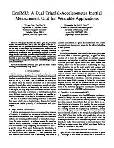
1

Acceleration (m/s 2 )

Reference Raw Newton GD LM 0.5

0

-0.5 0

5

10

15

20 Time (s)

25

30

35

40

Fig.4. Comparison between the results of proposed method, GD and Newton Methods.

4.2. Results and Discussion

RMSE 

The dynamical model used in this paper for modelling of accelerometer output is shown in (14).

ae (k )  f  n(k ), ao (k ), ao (k 1)  , k  1,..., N

(14) Where

ae is the model output, n is the assumed

white noise, ao is the raw output of the accelerometer and N is the number of data. To determine the performance of the method, Root Mean Square Errors (as shown in (15)) is used. International Journal of Automotive Engineering

Where

2 1 N   ar  k   ae  k   N k 1

(15)

ar is the reference signal. In Table 1, the

performance of the proposed method is compared with Gradient Descent (GD) and Newton algorithms. Fig. 4 shows the outputs of neural networks trained by mentioned algorithms. Results show that the presented method has a better performance in lower numbers of iterations than trained networks by GD and Newton algorithms and better robustness against high frequency noises and environmental disturbances.




2262

The proposed inertial accelerometer calibration method can be used in the structure of advanced driver assistance systems such as brake assist and collision avoidance systems to estimate the vehicle acceleration. Table1. Performance comparison of the proposed method with Newton and GD methods.

Training Method

RMSE

Newton

0.0326

Number of Iterations 28

Gradient Descent (GD) LevenbergMarquardt (LM)

0.0893

1000 (Maximum)

0.0318

12

5. Conclusion Measurement of vehicle acceleration is one of the most important task to design of driver assistance systems and autonomous vehicles. Low-cost inertial MEMS-based sensors are widely used in the structure of vehicle navigation, but the error sources in the output of these sensors could have disruptive effects on the results. In this paper, a calibration algorithm based on neural network trained by LevenbergMardquardt was suggested to remove these effects. Results showed that presented method has an acceptable performance in real driving situations. The presented method can estimate the vehicle acceleration and is beneficial to use in the structure of advanced driver assistance systems.



2263



References [1]. Buehler, M., Iagnemma, K., Singh, S., The 2005 DARPA Grand Challenge: The Great Robot Race. Springer-Verlag, Berlin, Heidelberg, 2007. [2]. Pradalier, C., Hermosillo, J., Koike, C., Braillon, C., Bessiere, P., Laugier, C., The CyCab: a car-like robot navigating autonomously and safely among pedestrians. Journal of Robotics Autonomous Syst. 50 (1), 2005, pp. 51–67. [3]. Bishop, R., A survey of intelligent vehicle applications worldwide, Proc. IEEE Intelligent Vehicles Symposium, 2000, pp. 25–30. [4]. Seetharaman, G., Lakhotia, A., Blasch, E.P., Unmanned vehicles come of age: the DARPA grand challenge, Computer, 39 (12), 2006, pp. 26–29. [5]. Dehban, A., Sajedin, A., Menhaj, M., A cognitive based driver's steering behavior modeling, Proc. Int. Conf. on Control, Instrumentation, and Automation, 2016, pp. 390-395. [6]. Fernandez, S., Ito, T., Driver Behavior Based on Ontology for Intelligent Transportation Systems, Proc. Int., Conf., on Service-Oriented Computing and Applications, 2015, pp. 227-231. [7]. Petkov, P., Slavov, T., Stochastic Modelling of MEMS Inertial Sensors, Journal of Cybernetics and Information Technologies, 10(2), 2010, pp. 31-40. [8]. Aktakka, E., Najafi, K., A six-axis micro platform for in situ calibration of MEMS inertial sensors, Proc. Int. Conf. Micro Electro Mechanical Systems, 2016, pp. 243-246. [9]. Shen, S., Chen, C., Huang, H., A new Calibration Method for Low Cost MEMS Calibration Sensor Module, Journal of Marine Science and Technology, 18(6), 2010, pp. 819-824. [10]. Aydemir, G., Saranli, A., Characterization and calibration of MEMS inertial sensors for state and parameter estimation applications, Journal of Measurement, 45, 2012, pp. 1210-1225. [11]. Lu, S., Basar, T., Robust Nonlinear System Identification Using Neural-Network Models, Trans. Neural Networks, 9(3), 1998, pp. 407-429. [12]. Tutunji, T., Parametric System Identification Using Neural Networks,


[13].

[14].

[15].

[16].

[17].

[18].

[19].

[20].

[21].

[22].

[23].

Journal of Applied Soft Computing, 47, 2016, pp.251-261. Jiang, X., Mahadevan, S., Yuan, Y., Fuzzy Stochastic Neural Network Model for Stochastic System Identification, Journal of Mechanical Systems and Signal Processing, 82, 2016, pp. 394-411. Fu, Z., Xie, W., Luo, W., Robust On-line Nonlinear Systems Identification Using Multilayer Dynamic Neural Networks with Two-time Scales, Journal of Neurocomputing, 113, 2013, pp. 16-26. Tobiyama, S., Yamaguchi, Y., Shimada, H., Malware Detection with Deep Neural Network Using Process Behavior, Proc. Computer Software and Applications Conf., 2, 2016, pp. 557-582. Wu, J., An evolutionary multi-layer perceptron neural network for solving unconstrained global optimization problems, Proc. Computer and information Science Conf., 2016, pp. 1-6. Li, Y., Yang, X., Shi, L., Finite-time synchronization for competitive neural networks with mixed delay and nonidentical perturbations, Journal of Neurocomputing, 185, 2016, pp. 242-253. Vieria, F., Lee, L., A Neural Architecture Based on the Adaptive Resonant Theory and Recurrent Neural Networks, Int. Journal of Computer Science and Applications, 4(3), 2007, pp. 45-56. Pastukhov, A., Prokofiev, A., Kohonen self-organizing map application to representative sample formation in the training of the multilayer perceptron, St. Petersburg Polytechnical University Journal: Physics and Mathematics, 2(2), 2016, pp. 134-143. Atencia, M., Joya, G., Hopfield networks: from optimization to adaptive control, Proc. Int. Joint Conf. Neural Networks, 2015, pp. 1-8. Rijwani, P., Jain, S., Enhanced Software Effort Estimation using Multi Layered Feed Forward Artificial Neural Network Technique, Journal of Procedia Computer Science, 89, 2016, pp. 307-312. Levenberg, K., A method for the solution of certain problems in least squares, Quarterly of Applied Mathematics, 5, 1944, pp. 164–168. Marquardt, D., An algorithm for leastsquares estimation of nonlinear parameters,




[24].

[25].

[26].

[27].

2264

SIAM Journal on Applied Mathematics, 11(2), 1963, pp. 431–441. Burachik, R., Drummond, L., Iusem, A. Svaiter, B., Full Convergence of the Steepest Descent Method with Inexact Line Searches, Journal of Optimization, 32, 1995, pp. 137-146. Yan, J., Tiberius, C., Bellusci, G., Janssen, G., Feasibility of Gauss Newton Method for Indoor Positioning, Proc. Position, Location and Navigation Sym., 2008, pp. 660-670. Saini, L., Soni, M., Artificial neural network based peak load forecasting using Levenberg-Marquardt and quasi-Newton methods, Proc. Generation, Transmission and Distribution, 149(5), 2002, pp. 578584. Nuraini, K., Najahaty, I., Hidayati, L., Combination of singular value decomposition and K-means clustering methods for topic detection on Twitter, Proc. Advanced Computer Science and Information Systems Conf., 2015, pp. 123128.

