tion matrix (that represents intrinsic sensor parameters) and a motion matrix ... Right: Inertial sensor unit composed of at least more than three sensor elements to ...
Factorization-Based Calibration Method for MEMS Inertial Measurement Unit Myung Hwangbo
Takeo Kanade
The Robotics Institute, Carnegie Mellon University 5000 Forbes Avenue, Pittsburgh, PA, 15213, USA {myung, tk}@cs.cmu.edu
Abstract— We present an easy-to-use calibration method for MEMS inertial sensor units based on the Factorization method which was originally invented for shape-and-motion recovery in computer vision. Our method requires no explicit knowledge of individual motions applied during calibration procedure. Instead a set of motion constraints in the form of an innerproduct is used to factorize sensor measurements into a calibration matrix (that represents intrinsic sensor parameters) and a motion matrix (that represents acceleration or angular velocity). These motion constraints can be collected quickly from a lowcost calibration apparatus. Our method is not limited to just triad configurations but also applicable to any coordination of more than three sensor elements. A redundant configuration has the benefit that all the calibration parameters including biases are estimated at once. Simulation and experiments are provided to verify the proposed method.
I. I NTRODUCTION MEMS-based inertial sensors with low cost and affordable performance are becoming prevalent in many applications such as land vehicles, air vehicles, and hand-held devices. An Inertial Measurement Unit (IMU) composed of such sensors is, for example, used solely for body attitude estimation in game controllers, or integrated with other sensors to either improve vehicle state estimation [1] or cope with intermittent loss of GPS data [2]. The low cost and small size of the inertial sensors encourage using redundant configurations that provide lower estimation variance as well as fault tolerance [3][4]. Sensor calibration prior to real use, however, remains tedious and becomes more complex as the number of sensor elements used increases. In calibration, obtaining the ground-truth reference is always one of the key and often costly processes. Because gravity force is an ideal reference for accelerometers, a mechanical platform has traditionally been used to either place an IMU at precisely known orientations or turn it at known constant speeds for gyroscope calibration [5][6]. Other types of equipment that can measure accurate reference motions, such as an optical tracking system, have also been used [7]. Recent work on IMU calibration, however, aims at eliminating the need for such an expensive calibration apparatus [8]. Skog and Händel [9] relaxed the requirement to know orientation angles in accelerometer calibration and presented a nonlinear method that minimizes the magnitude error in force recovery. They used a misalignment model of triad sensor configuration and it prevents to extend their
method to redundant configuration cases. The most relevant work to this paper is Voyles et al. [10] They proposed the shape-from-motion approach to force/torque sensor calibration based on the well-known Factorization method in the computer vision community [11]. The same basic principle is applicable to IMU calibration. When a camera or an IMU follows an affine linear model, measurements can be factorized as the product of two matrices: one corresponding to the object shape in computer vision and to the intrinsic configuration of sensor elements in the IMU, and the other corresponding to the camera motion in computer vision and to the motion (force or angular velocity) of the IMU. Since ambiguity still remains after the Factorization, calibration methods should provide a way to clear this ambiguity in order to recover the true intrinsic parameters. The main contribution of our work is to formulate an inertial sensor calibration problem to a reconstruction problem by the Factorization approach. By virtue of a generalized description of the sensor configuration, our method is not just limited to triad configurations but also applicable to redundant configurations where sensors’ biases can be simultaneously estimated. No prior knowledge of the sensor configuration is necessary for our method. The rest of the paper is organized as follows. Section II describes the Factorization method. Section III explains how to resolve the ambiguity for true reconstruction. Section IV shows full steps of calibration procedure. And finally Section V presents simulation and experiment results. II. FACTORIZATION : S HAPE -F ROM -M OTION A. Affine Linear Sensor Model An inertial sensor element based on MEMS-technology has a good linear input-output response with a non-zero output for null input (See Figure 1). Nonlinearity of ADXL203 used in our experiments is, for example, typically less than 0.5% of full scale [12]. Since no difference exists between accelerometers and gyroscopes in our calibration method, either force or angular velocity that the inertial sensor experiences is referred to as a motion. The measurement of a single sensor element, z, for a motion f s is expressed as z = a fs + b (1)
s3
fs
C. Factorization for Redundant Configuration (n ≥ 4)
z z
b
f (or w) a
{M}
s2
s1
fs
sn
Fig. 1. Left: Linear inertial sensor model with the gain s and the bias b. Right: Inertial sensor unit composed of at least more than three sensor elements to measure either accelerations or angular velocities in 3D.
where a is the gain and b is the bias of the element. Suppose n sensor elements are assembled as a unit to measure 3D motions. The output of each element in the unit is rewritten in a vector form for i = 1, . . . , n. �
zi = f si + bi
(2)
So, the motion f is projected on each sensitivity axis s i of which magnitude is the same as the gain a i = �si �. B. Measurement Matrix Let Z be a measurement matrix after m different motions are applied to the sensor unit of total n elements. z ij is the output of the sensor element j for the motion f i . Replacing it with the linear sensor model (2) gives ⎤ ⎡ � f1 s1 + b1 f1� s2 + b2 · · · f1� sn + bn ⎢f2� s1 + b1 f2� s2 + b2 · · · f2� sn + bn ⎥ ⎥ ⎢ (3) Z=⎢ ⎥ .. .. .. ⎦ ⎣ . . . � � � fm s1 + b1 fm s2 + b2 · · · fm sn + bn The measurements Z are rewritten as the product of two matrices, Fb and Sb , which are called a true motion matrix and a true shape matrix, respectively. ⎤ ⎡ � f1 1 ⎢f2� 1⎥ � ⎥ s1 s2 · · · sn ⎢ (4) Z = ⎢ . .. ⎥ b b · · · b ⎣ .. 2 n .⎦ 1 � 1 fm �
� S F 1 = (5) = Fb Sb b Note that the subscript b is intended to clarify that the shape matrix Sb includes biases. The goal of calibration is to identify the true shape matrix S b from a set of measurements Z generated in a principled way. The sensitivity axes in S reveal how sensor elements are aligned to each other in the unit. If all motions F could be known by any means, then calibration process would become trivial by taking the pseudo-inverse of the known motion matrix. Sb = F†b Z
(6)
The approach taken in this paper is, however, to obtain Sb without explicit knowledge about motions applied during calibration.
Factorization is a reverse process that decouples a given measurement matrix back into two parts: those which are associated with applied motions and intrinsic sensor element configuration. Let p denote the number of model parameters for a sensor element. It is the same as the row size of S b (p = 4 for affine linear model). Assume there exists at least p sensor elements in the unit and at least p motions are applied (n ≥ p, m ≥ p). From (5), the rank of the measurement matrix Z should be p from the minimum rank in the (m × p) motion matrix and the (p × n) shape matrix. It is called the proper rank constraint [13]. The first step is to enforce this constraint on Z, which is usually violated by measurement noise. It is achievable by Singular Value Decomposition (SVD) which produces the following unique decomposition Z
= U Σ V�
(7)
where U is an (m× m) orthonormal matrix, Σ is an (m× n) diagonal matrix, and V is an (n × n) orthonormal matrix. closest to Z in the sense of From SVD a rank-p matrix Z Frobenius norm is Z
Σ V � = Up Σp Vp� = U
(8)
is composed of the first p columns of U, Σ is the where U first (p × p) diagonal block matrix of Σ, and V is the first p columns of V. It is possible to obtain a canonical form of motion and b , that are not true matrices yet. This b and S shape matrices, F is because any (p×p) invertible matrix A and its inverse can be inserted between these two matrices and can also produce the same measurement matrix.
�) = F b S b = (U Σ) ( Σ V (9) Z −1 b ) = Fb Sb b A) (A S (10) = (F The key step in our calibration method is, therefore, to resolve ambiguity A from a set of motion constraints deliberately designed in the experiments. In other words, SVD b which are b and S gives a projective reconstruction of F ambiguous up to the transformation A and then the known geometric relation between true motion vectors in F b can determine A. The next section will describe this step in detail for accelerometer and gyroscope units. Finally, the projective reconstruction is upgraded to a metric reconstruction once A is found. Fb Sb
bA = F b = A−1 S
(11) (12)
D. Factorization for Triad Configuration (n = 3) Most IMUs have three sensor elements, which are the minimum number needed to sense 3D motions. Since the Factorization method is applicable only if n ≥ p, the bias {bj } needs to be known a priori in order to decrement the
preferred to have more constraints of different natures. The following describes how to determine A from a set of motion constraints in (15). A. Redundant configuration: n ≥ 4 and p = 4
Fig. 2. An IMU is mounted inside a calibration apparatus called a universal right angle iron. The iron has six surfaces that are square and parallel to each other within 0.002" per 6". When the iron is placed on a flat surface it is simple and easy to apply either orthogonal motions or motions in completely opposite directions to the IMU.
number of sensor model parameters. The bias-compensated measurement D is then used as input for the Factorization. ⎡ �⎤ f1 ⎢f2� ⎥
� ⎢ ⎥ D = ⎢ . ⎥ s1 s2 · · · sn = F S (13) ⎣ .. ⎦ T fm
where dij = zij − bj = fi� sj . Now the shape matrix S contains sensitivity axes only. Every step in the Factorization is identical except that p = 3 and the row and column sizes of A decrease by one. Regarding gyroscopes, it is trivial to estimate the biases because they are equal to sensor measurements when no motion is given (b j = zij when fi = 0). For accelerometers, it is difficult to determine the biases since gravity is always acting on the sensors. One possible solution appropriate for our calibration method is to apply two motions of the same magnitude but in completely opposite directions. � z1j = f1� sj + bj z1j + z2j (14) f1 = −f2 ⇒ bj = � 2 z2j = f2 sj + bj The gravity forces applied to the unit are completely opposite when the iron shown in Figure 2 is flipped over. It is noteworthy that one extra sensor element in the unit enables simultaneous estimation of all calibration parameters including biases. III. M ETRIC R ECONSTRUCTION In our calibration method, a set of following constraints between true motions in the form of an inner-product is elaborated to identify A for a metric reconstruction. fi� fk = hik
(15)
Note that explicit knowledge of the individual true motions, fi and fk , is not necessary. Relative or partial information about them is sufficient instead. It includes, for example, the magnitude of the motion (h ii = �fi �2 ) or a pair of orthogonal motions (h ik = 0). The universal right-angle iron in Figure 2 makes it convenient to collect an abundance of motions which are constrained by the iron’s parallel or square surfaces. Theoretically no apparatus is needed for accelerometer calibration in our method; however, it is
Let A be a non-singular (4 × 4) matrix composed of three blocks as � �
C a4 (16) A = A13 a4 = u� where A13 a (4 × 3) matrix, a4 is a (4 × 1) vector, C is a (3 × 3) square matrix, and u is a (3 × 1) vector. Firstly, a4 is obtainable directly without using any constraint. From (11) and (16), we have
�
� b A = F b A13 a4 = F 1 F (17) The last column of F b is fixed as a vector of one and a 4 is the only part that is associated with it in A. Therefore, a 4 is computed in a least square manner by taking the pseudo b. inverse of F −1 F � † 1 = (F � a4 = F b Fb ) b 1 b
(18)
Secondly, Q = A13 A� 13 will be found as an intermediate step from a set of motion constraints. The first three columns of (11) are rewritten as fi = A� 13 fb,i
for i = 1 . . . m
(19)
where fi is a (3 × 1) vector and fb,i is a (4 × 1) row vector of b . Substituting (15) with (19) produces one linear equation F (20) for an unknown (4 × 4) symmetric matrix Q. fi� fk
= fb,i� A13 A� 13 fb,k � = f Q fb,k = hik b,i
(20)
Let q be a (10 × 1) vector consisting of upper triangular elements of Q. A set of linear equations L b can be constructed by stacking � b for q per one motion constraint. 1 �b ( fb,i , fb,k ) q = hik
(21)
Lb q = h
(22)
At least 10 linearly independent constraints are needed to solve q uniquely. For redundant constraints, a least square solution for q is obtained from the pseudo inverse of L. Finally, A13 is uncovered from Q. Note that Cholesky decomposition is not applicable here because Q is generated from the non-square matrix A 13 . Instead, the relation between C, u and block matrices in Q needs to be derived first. � � Q0 q1 CC� Cu � Q = A13 A13 = (23) ≡ � (Cu)� u�u q1 q2 where Qo is a (3 × 3) symmetric matrix, q1 is a (3 × 1) vector, and q 2 is a scalar. The block matrices in Q are not 1 � (x, y) = [ x y , x y , x y , x y , x y + x y , x y + 1 1 2 2 3 3 4 4 1 2 2 1 2 3 b x 3 y2 , x 3 y4 + x 4 y3 , x 1 y3 + x 3 y1 , x 2 y4 + x 4 y2 , x 1 y4 + x 4 y1 ]
independent from each other but related by the following equation from the relation (Cu)� (CC� )−1 (Cu) = u�u. −1 q� 1 Q0 q1 = q2
(24)
By comparing the block matrices between the last equality in (23), C is obtained from Cholesky decomposition on Q 0 up to a rotation matrix R, and then u is computed from C and q1 . C = chol(Q0 ) u = C−1 q1
(a)
(b)
(c)
(d)
(e)
(f)
(g)
(h)
(i)
(j)
(25) (26)
The rotation ambiguity on C in the metric reconstruction is natural since it reflects on the fact that no coordinate system is ever defined for sensitivity axes. B. Triad configuration: n = p = 3 The biases b are assumed estimated separately as described in the previous section and subtracted from the measurements to use D instead of Z. The reconstruction from motion constraints is more straightforward because Q is generated from a (3 × 3) square matrix A. f � fk = f � AA� f� Q fk = hik (27) fk =
Fig. 3. Top row: Accelerometer unit inside the iron experiences gravity in many different directions. The gravity directions applied to accelerometers in (a), (b), and (c) are orthogonal to each other. Bottom row: The iron is rotated on top of a flat base by surface contact. The motions (angular velocities) applied in (f), (g), and (h) are orthogonal to each other. One precise amount of rotation is additionally required to decide the global scale β. For example, 90◦ rotation between (i) and (j) is achievable by aligning the iron with a straight ruler.
A set of linear equations L is obtained and solved for a (6 × 1) vector q composed of upper triangular elements of Q. 2 At least six constraints are needed for a unique q. fk ) q = hik −→ L q = h (28) �( fi ,
IV. C ALIBRATION P ROCEDURES
i
i
i
Finally, A is determined up to a rotation matrix R by Cholesky decomposition, A = chol(Q). C. Special cases One interesting case is that {h ik } are all identical. This occurs, for example, when the magnitude of gravity force is the only constraint for accelerometer calibration (�f i � = 1g). Because L loses one rank in this case, q from (22) is not unique any more but undetermined by α. q = qp + α qn
(29)
where qp is a vector in the column space of L and q n is a vector in its null space. The unknown scale α can be found by inserting (29) back into the block constraint of Q (24) which has not been used so far. It yields a four-order polynomial for α and only one of the polynomial roots is a valid real solution. For triad configuration, this is not the case since L remains full-rank. Another practical case is h = 0 when only orthogonal constraints are used for calibration. The q is in the onedimensional null space of L with an arbitrary scale β. q = β qn
(30)
It indicates that no constraint associated with the magnitude of a motion is involved so the gains {�s j �} of sensor elements cannot be extracted. One reference motion involved with the magnitude can determine an unknown global scale β. See Figure 3 (i)-(j). 2 �(x, y) = [ x y , x y , x y , x y + x y , x y + x y , x y + 1 1 2 2 3 3 1 2 2 1 2 3 3 2 1 3 x 3 y1 ]
The motion constraint (15) appropriate for our factorization method can be obtained easily with the assistance of precise measuring instrument such as a universal right-angle iron in Figure 2. A low-cost and easy-to-use calibration procedure appropriate for low-cost sensors can be implemented by this type of off-the-shelf product instead of specialpurpose expensive calibration equipment. The iron has six surfaces that are square and parallel to each other within 0.002" per 6". It can provide a more precise angular relation than the resolution of conventional MEMS-based sensors so that motions based on this device are sufficient to serve as ground-truth. An IMU is mounted inside the iron and its orientation with respect to the iron can be changed if more constraints are needed. When the iron is placed on a flat hard surface it is convenient to apply either orthogonal motions or motions in completely opposite directions to the IMU. A wealth of calibration data can be collected within a minute by turning the iron on every surface as shown in Figure 3. A. Accelerometer Unit Gravity is an ideal reference motion to calibrate an accelerometer unit. It is the only motion used in our calibration procedure. Let the motion f be normalized by gravity. Motion constraint types available from the right-angle iron are magnitude (h ii = 1), orthogonality (h ik = 0), and opposite (hik = -1). Therefore, more than the minimum constraints, which are 10 for n ≥ 4 and 6 for n = 3, are quickly obtained by flipping the iron on every surface. One possible standard procedure is summarized as depicted in Figure 3. 1) Install the IMU inside the iron. 2) Put the iron on its six surfaces by various turns. 3) Place the iron in other orientations if more data are needed.
z
For triad configuration, opposite motions are used separately for bias estimation in (14). In redundant cases, theoretically knowledge of true motions is completely relaxed except for the magnitude. Though no apparatus is even needed, it is recommended to use as many different constraint types as possible for the lower variance of parameter estimation. B. Gyroscope Unit The right-angle iron containing the gyroscope unit is rotated by hand on a surface contact with a clean flat bed. Sinusoidal motion is preferred for continuous smooth measurement data. This rotating motion is repeated with more than three orthogonal surfaces. From these experiments, the magnitude of angular velocity is unknown and orthogonality is the only available constraint type (h ik = 0). The global scale β remains undetermined as discussed in (30). One more experiment is therefore added to have the gyroscope unit rotate for a known rotation amount as shown in 3 (i)-(j). The following is the entire steps for gyroscope calibration. 1) 2) 3) 4) 5)
Install the IMU inside the iron. Rotate the iron with three orthogonal surfaces. Repeat previous steps with different IMU orientation. Rotate the iron Δθ for time T . Set the R in (25) so that the last motion f m is aligned with [1 0 0]� Because three linearly independent constraints are available per one fixed IMU mounting, the same experiment needs to be repeated with different IMU orientations with respect to the iron until enough constraints are collected. ⎡ ⎤ Δθ � t=T � t=T ⎢ 0 ⎥
� �† −1 ⎢ Sb z(t) dt = ⎣ ⎥ fb (t) dt = β (31) 0 ⎦ t=0 t=0 ∗ The rotation ambiguity R in the metric reconstruction is set in a way that the axis of Δθ rotation is aligned to one of coordinate axes. The global scale β can then be computed from the integration of measurements (31). C. Nonlinear optimization Once the true shape matrix is obtained, it is possible to refine it through a global minimization step. The least square nonlinear optimization provides a maximum likelihood estimator that guarantees the best estimation when measurement noise is Gaussian. The cost function is the squared sum of errors in the motion constraints. The applied motion is computed when the measurement z i and the sensor �
vector � † (zi − b). shape matrix Sb are given, fi = S � C= (fi� fk − hik )2 ��
�2 � (zi − b)� S� (S S� )−2 S (zk − b) − hik = Because the nonlinear method is sensitive to an initial condition, the solution from the linear method described in all previous sections can serve as a good initializer for it. The Levenberg-Marquardt or Gauss-Newton algorithm is a standard technique for implementation.
1500
s2
1400 1300 1200 1100
s1
{M}
1000
y
s3
900 800 700
s4
x
600 500
0
500
1000
1500
2000
2500
3000
Fig. 4. Left: The sensor configuration composed of two dual-axis accelerometers, total of n = 4, used in the simulation. Right: Experimental data from the accelerometer triad (n = 3) collected after placing the iron on six surfaces by turns. 2000 1800 1600 1400 1200 1000 800 600 400 200 0
0
100
200
300
400
500
600
700
700
800
900
1000
1100
50
600
0
500
+
[ST]|
400
-50 -100
300 -150
200
-200
100
-250
0 -100 0
20
40
60
80
100
120
140
160
-300 0
20
40
60
80
100
120
140
160
Fig. 5. Top: Experimental data from the gyroscope triad via sinusoidal rotation to the iron on its three orthogonal surfaces respectively. Bottom: Experimental data used for the last step of gyroscope calibration procedure to decide α. In the bottom right figure, the area enclosed by the curve should be the same as a precisely given rotation amount.
V. S IMULATION AND E XPERIMENTAL R ESULTS In simulation two dual-axis accelerometers like ADXL203, total of n = 4, are assumed in the unit as illustrated in Figure 4. The first dual-axis unit is oriented 45 ◦ off from the second one. Data are simulated under the same conditions as our real hardware targeted for UAV application [14] where 10-bit A/D converters sample the accelerometers at 50Hz. The data is digitized between 0 to 2047 which corresponds to −2.5g ∼ 2.5g. The data is generated with nominal sensor parameters from its product specifications and is corrupted by Gaussian noises of two different variances. The variance σ = 0.7 is an actual variance of accelerometers present in our laboratory-made IMU in Figure 6. The unit is placed at 20 different orientations and 10 measurements for each orientation are collected. A total of 200 gravity magnitude constraints are used in this simulation. Table-I shows estimation errors in biases b, gains �s i �, and angles between sensitivity axes. Because the Factorization method assumes noise-free measurement, it works more efficiently for less noisy data. The nonlinear optimization step starts with initial sensor parameters obtained from the Factorization method and it makes the RMS error of the
TABLE I
E STIMATION ERROR OF SHAPE MATRIX Sb FOR FOUR ACCELEROMETERS (n = 4) IN F IGURE 4 (S IMULATION )
Bias (volt)
Gain (volt/g)
Angle (deg)
Cerr
Ground truth b1 = 2.5 b2 = 2.5 b3 = 2.5 b4 = 2.5 �s1 � = 1.0 �s2 � = 1.0 �s3 � = 1.0 �s4 � = 1.0 ∠s1 s2 = 90.0 ∠s1 s3 = 90.0 ∠s1 s4 = 45.0 ∠s2 s3 = 90.0 ∠s2 s4 = 90.0 ∠s3 s4 = 45.0
Factorization (linear) (σ = 1.5) (σ = 0.7) 0.00139 0.00063 0.00122 0.00079 0.00113 0.00104 0.00177 0.00095 0.00236 0.00173 0.00150 0.00123 0.00187 0.00141 0.00325 0.00198 -0.16495 -0.05283 -0.35232 -0.22175 -0.08894 -0.04328 -0.18666 -0.16611 -0.37098 -0.27205 -0.07601 -0.00955 0.00175 0.00042
Nonlinear (σ = 0.7) 0.00019 0.00035 0.00000 -0.00014 0.00021 0.00029 0.00012 -0.00034 -0.02079 -0.02585 0.00030 -0.02502 0.02135 -0.02103 1.141×10⁻⁷
TABLE II
T HE RECOVERED SHAPE MATRIX S FOR THREE GYROSCOPES IN OUR LABORATORY- MADE IMU (E XPERIMENT )
Bias (volt) Gain (volt/rad/s) Angle (deg) Cerr
Nominal b1 = 2.5 b2 = 2.5 b3 = 2.5 �s1 � = 0.7162 �s2 � = 0.7162 �s3 � = 0.7162 ∠s1 s2 = 90.0 ∠s2 s3 = 90.0 ∠s1 s3 = 90.0 0.0163
Factorization 2.3061 2.5525 2.3734 0.7109 0.7303 0.7391 91.920 89.362 92.167 0.0026
Nonlinear 2.3063 2.5517 2.3731 0.7287 0.7403 0.7230 90.807 89.900 89.239 1.167×10⁻⁷
motion constraints drop dramatically. Figure 5 shows real measurement data from the gyroscope experiment on our laboratory-made IMU. Since it has triad configuration, the biases are estimated in a static condition. Six sets of sinusoidal measurement data are collected from two different IMU orientations using three orthogonal iron surfaces. One precise 90 ◦ turn is also given by aligning the iron with a straight ruler. Because any two sampled measurements associated with orthogonal iron surfaces are constrained, we now have enormous orthogonal constraints. The estimated parameters of three gyroscopes are listed in Table II. The final solution is refined much by the nonlinear optimization. It is because the best estimate for the biases, computed separately in the Factorization method, is searched together with the other parameters. VI. C ONCLUSION We have developed an easy-to-use calibration method for MEMS inertial sensors based on the Factorization method. It relaxes explicit knowledge of reference motions and recovers the intrinsic shape of a sensor unit from a set of motion constraints. Abundant constrained motions can be easily collected from low-cost apparatus such as a universal rightangle iron. The complexity of the calibration method remains
Fig. 6. Our laboratory-made IMU consists of two dual-axis accelerometers (ADXL-203) and three single-axis gyroscopes (ADXRS-150). It needs to be calibrated with respect to a camera for UAV vision application [14].
the same no matter how many sensor elements are in the unit. A redundant configuration is more appropriate for our method because all sensor parameters can be estimated simultaneously. Real implementation is also easy and simple provided basic linear algebra libraries. Once the internal shapes of sensor elements are found, the external relation (Rext , text ) with other coordinates such as camera or vehicle body frame can be estimated separately. R EFERENCES [1] E. Nebot and H. Durrant-Whyte, “Initial calibration and alignment of low-cost inertial navigation,” Journal of Robotic Systems, vol. 16, no. 2, pp. 81–92, 1999. [2] S. Sukkarieh, P. Gibbens, B. Grocholsky, K. Willis, and H. F. DurrantWhyte, “A low-cost, redundant inertial measurement unit for unmanned air vehicles,” The International Journal of Robotics Research, vol. 19, no. 11, pp. 1089–1103, 2000. [3] M. E. Pittelkau, “RIMU misalignment vector decomposition,” in AAS/AIAA Astrodynamics Specialist Conference and Exhibit, Aug. 2004. [4] S. Y. Cho and C. G. Park, “A calibration technique for a redundant imu containing low-grade inertial sensors,” ETRI Journal, vol. 27, no. 4, pp. 418–426, 2005. [5] R. M. Rogers, Applied Mathematics in Integrated Navigation Systems (AIAA Education Series), 2nd ed. AIAA, 2003. [6] J. J. Hall and R. L. W. II, “Inertial measurement unit calibration platform,” Journal of Robotic Systems, vol. 17, no. 11, pp. 623–632, 2000. [7] A. Kim and M. F. Golnaraghi, “Initial calibration of an inertial measurement unit using an optical position tracking system,” in IEEE Position Location and Navigation Symposium (PLANS 2004), Apr. 2004, pp. 96–101. [8] Z. Wu, Z. Wang, and Y. Ge, “Gravity based online calibration for monolithic triaxial accelerometers’ gain and offset drift,” in Proc. 4th World Congress on Intelligent Control and Automation, vol. 3, June 2002. [9] I. Skog and P. Händel, “Calibration of a MEMS inertial measurement unit,” in XVII IMEKO World Congress, Rio de Janeiro, Brazil, Sept. 2006. [10] R. M. Voyles, J. D. Morrow, and P. K. Khosla, “Shape from motion approach to rapid and precise force/torque sensor calibration,” in Int’l Mechanical Eng Congress and Exposition, Nov. 1995. [11] C. Tomasi and T. Kanade, “Shape and motion from image streams under orthography: a factorization method,” International Journal of Computer Vision, vol. 9, no. 2, pp. 137–154, 1992. [12] Analog Device, “ADXL203 precision dual-axis iMEMS accelerometer,” in Data Sheets, Mar. 2006. [13] R. I. Hartley and A. Zisserman, Multiple View Geometry in Computer Vision, 2nd ed. Cambridge University Press, 2004. [14] T. Kanade, O. Amidi, and Q. Ke, “Real-time and 3D vision for autonomous small and micro air vehicles,” in IEEE Conf. on Decision and Control, Dec. 2004, pp. 1655–1662.