the same item family. Glas and van der Linden (2001) suggest a Bayesian hierarchical model to analyze data involving item families with multiple-choice items.
RESEARCH REPORT August 2003 RR-03-23
Calibration of Polytomous Item Families Using Bayesian Hierarchical Modeling
Matthew S. Johnson Sandip Sinharay
Research & Development Division Princeton, NJ 08541
Calibration of Polytomous Item Families Using Bayesian Hierarchical Modeling
Matthew S. Johnson Baruch College, New York, NY Sandip Sinharay Educational Testing Service, Princeton, NJ
August 2003
Research Reports provide preliminary and limited dissemination of ETS research prior to publication. They are available without charge from: Research Publications Office Mail Stop 7-R Educational Testing Service Princeton, NJ 08541
Abstract
For complex educational assessments, there is an increasing use of item families, which are groups of related items. However, calibration or scoring for such an assessment requires fitting models that take into account the dependence structure inherent among the items that belong to the same item family. Glas and van der Linden (2001) suggest a Bayesian hierarchical model to analyze data involving item families with multiple-choice items. This paper extends the model to take into account item families with polytomous items and designs a Markov chain Monte Carlo (MCMC) algorithm for the Bayesian estimation of the model parameters. The hierarchical model, which accounts for the dependence structure inherent among the items, implicitly defines the family response function for the score categories. This paper suggests a way to combine the family response functions over the score categories to obtain a family score function, which is a quick graphical summary of the expected score of an individual with a certain ability on an item randomly generated from an item family. This paper also suggests a method for the Bayesian estimation of the family response function and family score function. This work is a significant step towards building a tool to analyze data involving item families and may be very useful practically, for example, in automatic item generation systems that create tests involving item families.
Key words: Hierarchical model; Markov chain Monte Carlo; automatic item generation; family response function; family score function; item score function
i
Acknowledgements
The research was supported by Educational Testing Service Research Allocation project 884.12. The authors thank Andreas Oranje, Isaac Bejar, Randy Bennett, Paul Holland, Alina von Davier, Hariharan Swaminathan, Shelby Haberman, and David Williamson for their helpful comments about the work and Kim Fryer for her help with proofreading. In addition, the authors gratefully acknowledge the National Center for Education Statistics for allowing access to the NAEP Mathematics Online data.
ii
1. Introduction
Any large-scale testing program requires a rich collection of items. While efforts to create new items are laborious for multiple-choice (MC) items, the same for complex constructed-response (CR) tasks are even more challenging. Due to the effort, expense, and occasionally inconsistent item quality associated with traditional item production, there is an increasing interest in using item models (Bejar, 1996) to guide production of items, automatically or manually, with similar conceptual and statistical properties. Items produced from a single item model, whether by automatic item generation (AIG) systems (Irvine & Kyllonen, 2002) or by rigorous manual procedures, are related to one another through the common generating model, and therefore constitute a family of related items. Naturally, it is necessary and beneficial to use calibration models that account for the dependence structure among the items from the same item family. The works by Janssen, Tuerlinckx, Meulders, and De Boeck (2000) and Wright (2002) are initial attempts at building such models. Glas and van der Linden (2001) suggest one such model for dichotomous items that is more general. The model assumes the item parameters of a three-parameter (3PL) logistic model (Birnbaum, 1968) to be normally distributed—the mean vector and the variance matrix of the normal distribution depend on the item model from which the item is generated. Glas and van der Linden’s model has the limitation that it cannot take into account families with polytomous items. This paper generalizes Glas and van der Linden’s model to take into account item families with those items as well. Further, this work designs a method to estimate the joint posterior distribution of the model parameters using the Markov chain Monte Carlo (MCMC) algorithm (Gilks, Richardson, & Spiegelhalter, 1996). The hierarchical model implies a family response function for each category for an item family. The family response function for score category k (assuming that the each item has K score categories) for an item family gives the probability that an individual with a given ability will score k on an item randomly generated from the item family. The idea is similar to that behind the family expected response function defined by Sinharay, Johnson, and Williamson (2003), who deal with families with dichotomous items. This paper suggests a way to combine the family response functions over the score categories to obtain a family score function, which is
1
a quick graphical summary of the expected score of an individual with a given ability to an item randomly generated from an item family. This work also suggests a way to compute estimates of the family response function and family score function and an approximate prediction interval around them using the Monte Carlo method and the output of the MCMC algorithm. The paper examines the performance of the hierarchical model using both true data and real data. The hierarchical model suggested here has the potential of immediate application to paper and pencil tests with items generated from item models either automatically or manually. Considering the fact that the present operational computerized adaptive tests use only MC items, our work may not be of any immediate help for computerized adaptive tests. However, it is possible to think of computerized adaptive tests with polytomous MC items, or, in the near future, even with CR items—this work will be helpful in that context. Another important issue with this document is the terminology used. There is no unanimous taxonomy in automatic item generation literature. What we call “item model” is also called “item template” (e.g., Deane & Sheehan, 2003), “schema” (Singley & Bennett, 2002), “item form,” etc., by other researchers. Similarly, what we call a “sibling” may be referred to as a “variant” or an “instance” or an “isomorph” or a “clone,” etc., elsewhere. And we refer to all the siblings generated from an item model as an “item family,” for the simple reason that the siblings are related to each other; the term item family is not meant to imply there is a “parent” item within each family. The next section provides a broad overview of the existing techniques for the analysis of data involving item families. Section 3 describes in detail one such model—the model generalizes Glas and van der Linden’s hierarchical model to account for polytomous item family data as well. Section 4 discusses estimation of the model parameters and the family expected response functions using the Markov chain Monte Carlo (MCMC) algorithm. Section 5 reports the results from a simulation study. Section 6 discusses the application of the model to a data set from the National Assessment of Educational Progress (NAEP). Finally, the paper concludes with a summary of the findings and thoughts on possible future directions.
2
2. Models for Item Families
There are three approaches for modeling data involving item families. The models all develop from standard item response theory (IRT) models for dichotomous and polytomous data. This paper uses the 3PL model (Birnbaum, 1968) to describe the response behavior of examinees to dichotomous MC items and the generalized partial credit model (GPCM; Muraki, 1992) to describe the response behavior of examinees to CR items. The 3PL model assumes that the probability an individual with ability θi correctly responds to item j is defined by the following equation Pj1 (θ) = P (Xij = 1|θi , aj , βj , cj ) = cj +
1 − cj . 1 + exp{aj (βj − θ)}
(1)
The parameter cj is called the asymptote, aj is the item’s discrimination, and βj is the difficulty of the item. Pj0 (θ) = 1 − Pj1 (θ) is the probability that an examinee with ability θi incorrectly responds to item j. The GPCM assumes that the adjacent category logits are linear in the examinee’s proficiency θi . Mathematically the GPCM probabilities for an item with K score categories (0, 1, . . . , K − 1) are defined by the following: Pjk (θi ) ≡ P (Xij = k|θi , aj , βj , δj0 , δj1 , . . . δjK−1 ) P exp{kaj (θi − βj ) − aj k`=0 δj` } = PK−1 Pk k=0 exp{kaj (θi − βj ) − aj `=0 δj` }
(2)
for k = 0, 1, . . . , K − 1, where aj is the item discrimination, βj is the overall difficulty for the item, and δjk is the k-th item-category step parameter. To ensure identifiability, set δj0 = 0 P and K−1 `=0 δj` = 0, which results in the need of estimating only (K − 2) parameters out of δj1 , δj2 , . . . δjK−1 to fit the GPCM. Note that the two-parameter logistic (2PL) model (Birnbaum, 1968) is a special case of this model with K=2 and no δ-parameter. Unrelated Siblings Model
The gold standard approach for modeling item response functions is to assume that each item is independent of all other items, regardless of whether they are siblings or not. The resulting model is called the unrelated siblings model (USM) as the item parameters of the sibling response 3
functions are assumed to be unrelated, or independent. The USM assumes that Xij , examinee i’s score to item j, follows a multinomial or binomial distribution with probabilities defined by the GPCM in (2) for CR items and probabilities defined by the 3PL model in (1) for MC items. The USM makes no other assumption about the item parameters. Although standard IRT software can fit the USM, the model has the disadvantage that each item has to be individually calibrated. In addition, this approach ignores the relationship between siblings in an item family and hence will provide standard errors of item parameters that are too large and will require larger sample sizes for acceptable calibration precision. Identical Siblings Model
Hombo and Dresher (2001) study the results of a model that assumes the same parameters and hence the same item response function for all items in the same item family. We call this approach the identical siblings model (ISM). This model assumes the same item parameters of the 3PL and GPCM for all items in the family. While this model can also be fit by standard software like PARSCALE (Muraki & Bock, 1997) or BILOG (Mislevy & Bock, 1982), it has the limitation that it ignores any variation between siblings and hence, in the face of such variations, provides biased estimates of the item parameters and is overconfident about the amount of information available to estimate examinee scores. Related Siblings Model
One way to overcome the limitations of the above-mentioned two methods is to apply the related siblings model (RSM), a hierarchical model that assumes a separate item response function for each item, but relates the siblings’ item parameters within a family using a hierarchical component (Glas & van der Linden, 2001). The method uses a mixing distribution to describe the relationship between items within the same item family, in much the same way that the mixing distribution on the student parameter θ in an IRT model is used to describe the dependence between item responses from the same examinee. One important point to note here is that the ISM and USM are limiting cases of the RSM. If the mixing distribution approaches a point mass (or the variances of the mixing distribution go to 0), then the RSM approaches the limit to the ISM. On the other hand, if the mixing distribution 4
approaches to the Lebesgue measure (or the variances of the mixing distribution go to ∞), then the RSM approaches the limit to the USM (Sinharay et al., 2003). While the advantage of the RSM is that it properly accounts for the variability among the items for the same item model, it has the disadvantage that there is no standard software for fitting this model. We use our own C++ program to fit the RSM in this work. Janssen et al. (2000) and Wright (2002) provide examples of such models. Glas and van der Linden (2001) suggest one such model for dichotomous items that is more general; the model starts from a 3PL model (Lord, 1980) and uses a normal mixing distribution to relate the item parameters belonging to the same family. The mean vector and the variance matrix of the normal mixing distribution depend on the item family from which the item is generated. All the above mentioned models have the limitation that they cannot take into account families with polytomous items. The next section discusses an example of an RSM that encompasses CR items as well. The model is an extension of the model by Glas and van der Linden (2001), is a Bayesian hierarchical model, and uses a normal mixing distribution to relate siblings. 3.
A Related Siblings Model for Polytomous Item Families
Suppose there are J items denoted by j = 1, 2, . . . J in a test, and that the j-th item is scored on a scale from 0 to (Kj − 1). Consider that the test is given to N examinees. Let I(j) be the item family of which item j is a member. Items j and k are siblings if they are members of the same item family, that is, if I(j) = I(k). We model MC items using the 3PL model defined in (1) and CR items using the GPCM defined in (2). To be able to use a normal mixing distribution on the item parameters, we apply the n o c transformations αj = log{aj } and γj = log 1−cj j . Assuming normality of αj and γj , both of which range from −∞ to ∞ (whereas aj ranges from 0 to ∞ and cj ranges from 0 to 1) is more reasonable. Recall that fitting a 3PL model requires estimating aj , βj , and cj for each item while fitting a GPCM requires estimating aj , βj , and any (Kj − 2) out of δj1 , δj2 , . . . δjKj −1 · Let (αj , βj , γj )0 if item j is an MC item ηj = 0 (αj , βj , δj1 , δj2 , . . . δ if item j is a CR item jKj −2 ) 5
(3)
be the item parameter vector for item j. The first component of the related siblings model, that defining the likelihood, is Xij ∼ Multinomial(1; Pj0 (θi ), . . . , PjKj −1 (θi )), where the probabilities Pj0 , . . . , PjKj −1 are defined in (1) or (2) depending on whether the item is an MC or a CR item. The population distribution for the latent abilities θi s is normal with mean µ and variance σ 2 . The hierarchical component of the related siblings model uses a normal mixing distribution to relate the item parameters of siblings as η j ∼ N (λI(j) , T I(j) ), where λI(j) =
(4)
(λaI(j) , λbI(j) , λgI(j) )0
if item j is an MC item
(λaI(j) , λbI(j) , λd I(j) , λd I(j) , . . . λd 1 2 K
j −2
I(j) )
0
(5)
if item j is a CR item
is the mean item parameter vector for family I(j), and TI(j) is the within-family item parameter covariance matrix for family I(j). Let λa denote the family discrimination parameters, and λb denote the family difficulty parameter. To fix the origin and scale (ensure identifiability), let µ = 0 and σ 2 = 1 (an alternative method would be to force sum-to-zero constraints on the first and second components of the item family mean parameter vectors λI(j) ). By integrating the individual item parameters out of the likelihood, the resulting model correctly accounts for the fact that responses by two individuals to the same item are correlated even when conditioning on the family parameter λI(j) and T I(j) . Also, as Sinharay et al. (2003) argue, ISM and USM are both limiting cases of the RSM. Family Response Function and Family Score Function
Note that by integrating the individual item parameter vectors η j out of the item response functions P j (θ), the RSM defines a new set of family response functions. Let Pk (θ | I) denote family I’s response function for category k, k = 0, 1, . . . , KI − 1. The family response function for category k is defined by Z Pk (θ | I) =
Pk (θ | η)dΦ(η | λI , TI ), η
6
k = 0, 1, . . . , KI − 1,
(6)
where Φ(.|., .) is the cumulative distribution function of the multivariate normal distribution and Pk (θ | η) is the k th category response function and is defined by (1) or (2) depending on whether the item is an MC item or a CR item. The family response function Pk (θ | I) defines the probability that an individual with proficiency θ will score k on a randomly selected item from family I. Sinharay et al. (2003), in the context of MC items, refer to the posterior expected function of the family response function as the family expected response function. Notice that an item family containing items with K score categories has the same number of family response functions. It is often desirable to examine a single function for each item family. Therefore, we define the family score function, m(θ|I), which describes the expected score on a randomly selected item from the I-th item family for an examinee with proficiency θ, as m(θ|I) =
K I −1 X
` × P` (θ|I),
(7)
`=0
where P` (θ|I) is defined in (6). A similar quantity exists for each individual item in each of the families. The item score function for item j, defined as mj (θ) =
K I −1 X
` × Pj` (θ),
(8)
`=0
describes the expected score on item j of an individual with proficiency θ, where Pj` (θ)s are defined in (1) or (2) depending on whether the item is an MC item or a CR item. Note that for a dichotomous item, the family score function becomes P1 (θ|I) and the item score function becomes Pj1 (θ). 4. Bayesian Estimation for the Related Siblings Model
Maximum likelihood estimation of the related siblings model requires the calculation of the joint likelihood function of the family parameters λI(j) s and T I(j) s given the observed data. Consistent estimation of these parameters would require marginalizing the likelihood with respect to both the examinee parameters θ and the individual item parameters η. The calculation of the family response function in (6) demonstrates how the item parameters could be integrated out of the response function. Suppose Λ denotes the collection of all λI(j) s, and T denotes the 7
collection of all T I(j) s. Now define the conditional likelihood of an examinee with proficiency θ given the family parameters λI(j) s and T I(j) s by taking the product over all item families L(θ | X, Λ, T ) =
Y
PxI (θ | I),
I
where xI is the examinee’s score to an item from family I, X is the vector of the scores of the examinee to all items, and PxI (θ | I) is defined in (6). It is not enough to simply integrate θ out of the examinee likelihood and take the product of the resulting terms to define the likelihood for the item family parameters. Doing so would require that item responses from different individuals to the same member of an item family be independent, when in fact they should be considered related to one another. However, by integrating the individual item parameters (αj , βj , γj )t out of the true joint likelihood, the resulting model correctly accounts for the fact that responses of two individuals to the same member from the same item family are correlated even when conditioning on the family parameter λI(j) and T I(j) . Maximizing the correct likelihood for the related siblings model would be an extremely difficult task requiring complex numerical integration techniques. We prefer to perform a Bayesian estimation of the model. Prior Distributions on Family Means and Variances
A fully Bayesian formulation of the model requires the specification of prior distributions for the model parameters λI(j) and T I(j) . We employ the use of conjugate prior distributions for these parameters as in Glas and van der Linden (2001). Assume independent multivariate normal prior distributions for the family mean item parameter vectors: λI(j) , λI(j) ∼ N (µλ , Vλ ) ·
(9)
In most cases we suggest using a diagonal matrix for Vλ , the prior covariance matrix of the mean item parameter vectors; in the absence of prior information, the diagonal elements of the matrix should be large, such as Vλ = 100I K , where I K is the K × K identity matrix. One situation where it is sensible to use an informative prior is when the item family is an MC family. In that situation, a good choice for a prior distribution would be one that places its
8
0.15
0.20 Y = (1 + exp(− λg))
0.25 −1
Figure 1: Probability density function for the random variable Y =
1 1+exp(−λg ) ,
where λg ∼
N (−1.386, 0.12 ).
mass around the point
µ ½ µλ = µa , µb , logit
1 No. of choices
¾¶0 ·
For example, in the case where the item family has five choices, a good option will be to use the prior mean µg = logit{0.2} = −1.386, and σg = 0.1. Figure 1 contains the density function of the transformed random variable Y =
1 , 1+exp(−λg )
where λg ∼ N (−1.386, 0.12 ). Note that the density
peaks approximately at 0.2 =
1 , No. of choices
and has almost all of its mass in the interval (0.15, 0.25). We assume independent inverse-Wishart prior distributions on the family variances: T −1 I(j) ∼ Wishart(W1 , W2 ).
(10)
The notation M ∼ Wishart(W1 , W2 ) implies that the density function of the p × p matrix M is proportional to µ
|M |
(W1 −p−1)/2
¶ 1 ¡ −1 ¢ exp − tr W2 M · 2
The above density is proper for W1 > p and finite everywhere if W1 > (p + 1). The prior in (10) implies that the prior mean of T −1 I(j) is W1 W2 , and that a priori there is information that is equivalent to W1 observations of the item parameter vector η j . 9
The Conditional Posterior Distributions and the MCMC Algorithm
Bayesian estimation requires the determination of the joint posterior distribution of all model parameters given the observed data. Because the posterior distribution requires the the evaluation of an intractable integral, we employ Markov chain Monte Carlo (MCMC) techniques (Gilks et al., 1996), specifically the Metropolis-Hastings algorithm (Metropolis, Rosenbluth, Rosenbluth, Teller, & Teller, 1953; Hastings, 1970) within a Gibbs sampler (Geman & Geman, 1984). The algorithm generates a sample of parameter values from a Markov chain that approximates the joint posterior distribution of the parameters of the model by drawing iteratively from the conditional posterior distribution of each model parameter. The Metropolis-Hastings-within-Gibbs algorithm draws the item parameters α, β, γ, δ and the ability variables θ from their respective conditional distributions as described in Patz and Junker (1999). Conditional on the item parameters η = set of all ηj s, where ηj is defined in (3), the I-th item family mean vector λI and covariance matrix TI are independent of θ and the observed data X. The conditional distributions of the λI s, which are independent over the families (i.e., over I), are given by ª ¢ ¡ © λI | η, TI ∼ N V I Vλ−1 µλ + JI TI −1 η I , V I , where
(11)
¡ ¢−1 V I = JI TI −1 + Vλ−1 ,
µλ and Vλ are the prior mean and variances of λI ’s respectively, ηI =
1 JI
X
ηj ,
j: I(j)=I
and JI is the number of members in item family I. The conditional distributions of the TI s, which are also independent over the families (i.e., over I), are given by TI | η, λ ∼ Inv-Wishart JI + W1 ,
X
j: I(j)=I
−1 · (η j − λI(j) )(η j − λI(j) )t + W2−1
10
(12)
The addition of the hierarchical component in the model amounts to additional sampling from normal and inverse Wishart distributions, which are both straightforward. Hence, the hierarchy of the model does not pose significant difficulties in the Bayesian estimation procedure. We look at a number of MCMC convergence diagnostics (Sinharay, 2003, and the references therein) to ensure the convergence of the MCMC algorithm before using the output for further inference. Estimating the Family Response Function
Monte Carlo integration provides a way to estimate the family response function defined in (6) and compute a 95% prediction interval for the family. The following steps describe the Monte Carlo procedure used for the estimation of the family response function and 95% prediction interval for the I-th family of items. 1. Generate a sample of size M from the joint posterior distribution of the hyper-parameters λI and TI . That is, draw [λI (t) , TI (t) ] ∼ F (λI , TI | X), t = 1, . . . , M · (t)
(t)
2. For each of the above M values of the hyper-parameters [λI , T I ] , draw n values of the item parameter vector η j from the conditional (prior) distribution of η j given λI (t) , and TI (t) , ((t−1)n+r)
ηj
∼ Φ(η j |λI , TI )
for r = 1, . . . , n and t = 1, . . . , M . 3. Set the ability at θ. (t)
4. For each of the M n draws η j obtained in step 2, compute the probability for category `, (t)
(t)
p` = P` (θ|η j ), for each of the item categories ` = 1, . . . , KI , where KI is the number of score categories for item family I. In addition calculate, the expected score function P (t) m(t) = ` × p` . 5. The averages of the above probabilities and expected score functions are Monte Carlo estimates of the posterior means of the category family response functions and the family score 11
function, E [P` (θ|I) | X] ≈ E [m(θ|I) | X] ≈
Mn X t=1 M n X
(t)
p` , m(t) ·
t=1
Sinharay et al. (2003) refer to the above estimated posterior means of family response functions as estimated family expected response functions while dealing with item families consisting of dichotomous items. (t)
6. The 2.5th and 97.5th percentiles of the M n probabilities p` and expected score functions m(t) form an approximate 95% prediction interval to attach with the estimates obtained in step 4. This prediction interval reflects the within family variance as well as the uncertainty in the family response functions. Steps 3 to 6 are repeated for a number of values of θ to obtain the estimated family response function for each category ` in item family I. We use M = 1, 000, n = 10, and 100 equidistant values of θ in the interval (-4,4) to estimate the function for all the analyses in this work. Note that the MCMC algorithm described earlier in this section provides a sample from an approximation of the posterior distribution. To obtain a sample of size M from the posterior distribution of λI and TI in step 1 above draw a subsample of size M from the output of the MCMC algorithm. Step 2 is simple because it only requires sampling from a multivariate normal distribution using the draws of λI and TI from step 1. So the estimation of the family response function is quite straightforward given the output from the MCMC and takes little additional time. 5. Example 1: A Simulation Study
In this section, a simulation study examines the performance of the RSM on data generated according to a family structure. Generating Data With Family Structure
The data generation process is very similar to that in Sinharay et al. (2003). We generate 16 item families: 5 families of two-category CR items (2PL), 5 families of MC items (3PL), and 12
six families of polytomous CR items (GPCM). Two families have three category items, 2 have four category items, and 2 have five category items. Each item family contains 10 items (siblings). We generate the values of the individual proficiency parameters θi s for N = 5, 000 examinees from a normal distribution with mean 0 and variance 1; each examinee receives 1 of 10 “forms” of the test. Each form contains 16 items; 1 item from each of the 16 item families. The first items in each family make up the first form; the second items from each family make up the second form, etc. Five-hundred randomly selected examinees respond to each form. This study generates item families in such a way that the resulting item parameters reflect the range of values typically observed in real life assessments. For example, from our experience, the discrimination parameters aj s usually fall between 0.5 and 1.5, and the data generator draws item families so that the item parameters will remain in that range. The data generator draws individual item parameters so that the within-family variance is one fifth as large as the between-family variance. Remembering that an RSM with very small within-family variance is essentially an ISM and an RSM with large within-family variance is essentially an USM (Sinharay et al., 2003), the ratio of within-family variance and the between-family variance used here makes data distinguishable from data generated by an USM or ISM. Analysis of the Simulated Data
To analyze the data, we use a Wishart prior distribution for the family precision matrix T −1 I with parameters W1 = kI + 1 and W2 =
W1 I , 10 kI
where kI is the number of item parameters
in the model for an item from family I (e.g., kI = 3 for a three-category item) and IkI is the kI × kI identity matrix. The prior mean of T −1 I , implied by the above choice of W1 and W2 , is (kI +1)2 IkI . 10
We apply the MCMC algorithm to approximate the posterior distributions of the model parameters. For this example, a number of convergence diagnostics (time-series plots, Gelman-Rubin convergence diagnostics, and the Brooks-Gelman multivariate potential scale reduction factor) indicate that a chain with 50,000 iterations is sufficient to ensure convergence. We discard the first 10,000 iterations as burn-in and use every 10th draw from the Markov chain, leaving us with 4,000 draws from the approximated posterior distribution of the model parameters. Figures 2 and 3 plot the approximated marginal posterior densities for the family 13
parameters λa and λb respectively. Figure 4 contains the approximated posterior density for the family guessing parameter for the five 3PL item families. The vertical line in each panel of the figures represents the average value of the true item parameters in that family. Family 1
0.5
Family 2
0.7
0.9
0.6
0.7
0.8
0.4
0.5
Family 4
0.6
0.0
0.1
0.2
0.3
λa
λa
λa
λa
Family 5
Family 6
Family 7
Family 8
−0.1
0.1
−0.2
0.5
Family 3
0.2
0.3
−0.4
0.0
0.4
0.8
0.4
0.8
1.2
0.2
0.4
0.6
0.8
λa
λa
λa
λa
Family 9
Family 10
Family 11
Family 12
0.2
0.6
0.0
0.5
1.0
−0.7
−0.5
−0.3
0.0
0.1
0.2
λa
λa
λa
λa
Family 13
Family 14
Family 15
Family 16
−0.4
−0.2 λa
−0.2
0.0 0.1 0.2
−0.3
λa
−0.1 0.0 λa
0.1
0.1
0.2
0.4
0.3
0.3
0.4
0.5
λa
Figure 2: Estimated posterior density functions of the family mean discriminations λa s for the simulation study.
Fourteen of the 95% credible intervals for the family discrimination parameters λa s contain the true parameter values (Figure 2). Families 8 and 10 are the only two families whose credible intervals do not contain the true value. The discrimination parameter of Family 8 is underestimated, and λa for Family 10 is overestimated. Further inspection reveals that these two families are MC item families. And the problem of obtaining a stable fit with the 3PL 14
Family 1
−1.7
−0.8
0.4
−1.0
−1.5
Family 2
−1.3
−0.35
Family 3
−0.20
−0.05
0.0
0.2
0.4
Family 4
0.6
0.3
0.5
0.7
λb
λb
λb
λb
Family 5
Family 6
Family 7
Family 8
−0.6
−0.4
1.2 1.4 1.6 1.8 2.0
−2.5
−2.0
−1.5
−1.0
−0.1
0.1
0.3
λb
λb
λb
λb
Family 9
Family 10
Family 11
Family 12
0.6
0.8
1.0
1.4
1.8
2.2
−0.2
0.0
0.2
0.4
−0.2
0.0
λb
λb
λb
λb
Family 13
Family 14
Family 15
Family 16
−0.8
−0.6
−1.0
−0.8
λb
−0.6
−1.3
λb
−1.1 λb
−0.9
−1.1
0.5
−0.9
0.1
−0.7
λb
Figure 3: Estimated posterior density functions of the family mean difficulties λb s for the simulation study.
model (Patz & Junker, 1999) occurs here as well, that is, item families modeled using the 3PL model not behaving as well as those modeled by a GPCM. Figure 3 indicates that the MCMC estimation algorithm does an excellent job of recovering the true values of λb s, the family difficulty parameters. In each of the 16 item families, the true value is contained within the 95% credible interval for that parameter. Figure 4 shows that the family guessing parameter for Family 8 is underestimated and the guessing parameter for Family10 is overestimated. Because of the near indeterminacy (especially for difficult items) of the 3PL model parameters, the overall effect of the under- or overestimation
15
Family 6
−3.0
−2.5
−3.0
Family 7
−2.0
−2.5
−1.5
−1.0
−8
−6
−4
−2
λg
λg
Family 8
Family 9
−2.0
−1.5
−1.0
−2.5
λg
−2.0
−1.5
0
−1.0
λg
Family 10
−1.6
−1.4
−1.2
−1.0
λg
Figure 4: Estimated posterior density functions of the family mean asymptotes λg s for the simulation study.
of the family parameters for Families 8 and 10 is minimal. This is evident in Figure 5, which contains the family score functions for the 16 simulated families, along with the true item score functions and the 95% prediction intervals for the families. The family score functions and 95% prediction intervals for Families 8 and 10 track the true item score functions quite well; only small portions of a single item score function extend beyond the 95% intervals in each of these two families. The two families that cause the greatest concern are the 7th and 14th item families. The family score function for Family 7 clearly has an asymptote that is different from the
16
2
4
0
2
4
0.8 0.0
0.4
P(θ)
0.8 0.4
P(θ)
−4 −2
−4 −2
0
2
4
−4 −2
0
2
Family 6
Family 7
Family 8
2
4
−4 −2
0
2
4
0.0
0.4
P(θ)
P(θ)
0.4 0.0
P(θ)
0.4 0.0
0.4
0
−4 −2
0
2
4
−4 −2
0
2
Family 9
Family 10
Family 11
Family 12
2
4
−4 −2
0
2
4
m(θ)
m(θ)
P(θ)
0.4 0.0
0.4 0.0
0
−4 −2
0
2
4
−4 −2
0
2
θ
Family 13
Family 14
Family 15
Family 16
4
−4 −2
0
2
4
1 0
−4 −2
θ
2
m(θ)
3
4 3 1 0
0.0
θ
2
2
m(θ)
2.0
m(θ)
1.0
2.0 1.0 0.0
0
4
4
θ
3.0
θ
3.0
θ
−4 −2
4
0.0 0.5 1.0 1.5 2.0
θ
0.0 0.5 1.0 1.5 2.0
θ
0.8
θ
0.8
θ
−4 −2
4
0.8
Family 5
0.8
θ
0.8
θ
0.8
θ
0.0
P(θ)
0.0
P(θ)
0
Family 4
θ
−4 −2
P(θ)
0.4 0.0
0.4 0.0
P(θ)
−4 −2
m(θ)
Family 3
0.8
Family 2
0.8
Family 1
0 θ
2
4
−4 −2
0
2
4
θ
Figure 5: The estimated family score functions (solid bold lines), corresponding 95% prediction intervals (solid lines), and the true item score functions (dashed lines) for the 16 item families in the simulated data set.
17
true item score functions. Once again this can be explained by the near indeterminacy between the difficulty and guessing parameters in the 3PL when the item (or family) is an easy one and noting that Family 7 consists of very easy items. The model is unable to distinguish between an item that is easy and one that is easy to guess. The model performs poorly for Family 14. There is a single item whose item score function is almost completely outside of the 95% prediction interval for the family. It is quite clear that the within family variance for this item is underestimated. Figure 6 contains the estimated posterior densities of the within family variance of the difficulty parameters (denoted as τb s) along with the simulated variance (true value of τb ). The true variance for the 14th family is the largest variance across all item families, but the approximated posterior density for this family is not substantially different from the other 15 families. This might be an indication that the amount of information in the observed data about this variance component is small relative to the amount of information provided by the prior distribution. This is not surprising given that the simulated data has only 10 items per item family, which is probably too few for estimating the within family variances. In addition to estimating family parameters, the MCMC algorithm also provides us with sampled values from the approximate posterior distribution of each examinee ability θi . Figure 7 contains the approximated posterior densities of five individual θi s—an individual with lowest raw score (0), an individual with the 25th percentile raw score (10), an individual with the median raw score (21), and an individual with highest raw score (28). The true values of the θi s are also shown using a vertical line. As expected, the means of the posterior distributions increase with raw score, and the posterior variances are largest for individuals with extreme scores (0 and 28). The 95% posterior credible intervals contain the true value of θ in all the five cases. Although the 95% credible interval (−1.76, − 0.44) for the individual with a raw score of 10 barely contains the true value of θ = −0.46, the posterior probability that the individuals θ is greater than −0.46 is only P r{θ > −0.46 | xi } = 0.03.
18
6.
Example 2: Analysis of the NAEP Mathematics Online Data
The National Assessment of Educational Progress (NAEP) is an ongoing educational survey administered by the National Center for Education Statistics (NCES). NAEP regularly reports on the progress of students in 4th, 8th, and 12th grade on a number of educational subjects (e.g., mathematics, reading). The Technology-based Assessment (TBA) project is a NAEP special study sponsored by NCES. The project is designed to explore the use of technology, especially computers, as a tool
Family 1
0.0
0.0
0.0
0.0
0.5
Family 2
1.0
1.5
0.0
0.2
0.4
Family 3
0.6
0.8
0.0
0.5
1.0
1.5
Family 4
2.0
0.0
0.5
1.0
τb
τb
τb
τb
Family 5
Family 6
Family 7
Family 8
1.0
2.0
0.0
0.5
1.0
1.5
2.0
0.0
0.5
1.0
1.5
0.0
0.4
0.8
τb
τb
τb
τb
Family 9
Family 10
Family 11
Family 12
0.5
1.0
1.5
0.0
0.4
0.8
0
1
2
3
4
0.0
0.2
0.4
0.6
τb
τb
τb
τb
Family 13
Family 14
Family 15
Family 16
0.2
0.4
0.6
0.0
0.5
τb
1.0
1.5
0.0 0.2 0.4 0.6 0.8
τb
τb
0.0
0.5
1.0
1.5
1.2
0.8
1.5
τb
Figure 6: Estimated posterior density functions of τb , the within-family variance component of the difficulties, for the simulation study.
19
f(θ|x)
0.4
−2
0
2
4
−4
−2
0
2
θ
θ
Raw score 15
Raw score 21
4
0.8
f(θ|x)
0.0
0.4
0.8 0.4 0.0
f(θ|x)
1.2
−4
0.0 0.4 0.8 1.2
Raw score 10
0.0
f(θ|x)
Raw score 0
−4
−2
0
2
4
−4
θ
−2
0
2
4
θ
0.3 0.0
f(θ|x)
0.6
Raw score 28
−4
−2
0
2
4
θ
Figure 7: Markov chain Monte Carlo approximated posterior densities for five of the simulated examinees.
to improve the quality and efficiency of assessments (National Center for Education Statistics, 2002). One of the studies included in the TBA project is the Mathematics Online (MOL) special study (Sandene, Bennett, Braswell, & Oranje, in press). The MOL study translates existing NAEP math questions into a computer delivery system to be used for the assessment of 4th and 8th grade students. The main goals of the MOL study were to: (a) determine how computer delivery affects the assessment of the examinees, (b) evaluate the abilities of 4th and 8th grade students to use a computer-based assessment, and (c) investigate the ability to create alternate versions of the assessment with the use of automatic item generation (AIG) (at Grade 8 only). In the following pages, we focus on the 8th grade MOL study. Data
This paper looks at responses of 3,793 examinees in Grade 8, distributed among four test forms (denoted M2–M5). Each test form has a block of common items (denoted MP) and an additional 26 items that varies, either in content or delivery method, across the four forms. Of the 20
26 items that varies across the forms, 16 are MC items and 10 are CR items. Of the 10 CR items, 5 items have two response categories each, 3 have three response categories each, and 2 have four response categories each. The items on Form M2 are the “parent” items. These are all written by humans and are representative of the NAEP mathematics item pool. Form M2 is a paper and pencil assessment much like the standard NAEP assessments (only shorter) with calculators provided for the students. The content of Form M3 is identical to Form M2. However, Form M3 is a computer-based assessment form and students must use an online calculator. Forms M4 and M5 contain 11 items (6 CR and 5 MC) that are identical to items on Forms M2 and M3. The remaining 15 items on Forms M4 and M5 are automatically generated (Singley & Bennett, 2002) from an item model based on the items on Form M2. However, these 15 items are not the same on Forms M4 and M5. So when compared to one another, Forms M4 and M5 have 11 identical items and 15 items that vary across the two forms. Forms M4 and M5 are paper and pencil forms with calculators provided where necessary, which is like Form M2. Table 1 summarizes the 26 item families; it provides the reader with the item types (e.g., 3PL, 3 category) in each family and with information about whether the items in Forms M4 and M5 were automatically generated. Sinharay et al. (2003) analyzed the MC items from this data set with Glas and van der Linden’s (2001) RSM. The later part of this section analyzes this data set using the RSM introduced in section 3 to demonstrate the practicality of the model. There are 26 item families, one corresponding to each item on Form M2. Although some of the items are identical across the forms, we treat the items on each form as distinct items. The 11 item families for items that do not vary across the forms give us some idea about the amount of tolerable variation (Rizavi, Way, Davey, & Herbert, 2002), as the variation is simply a combination of sampling and administration variation. The analysis ignores two pieces of information. The first is the common block of items in each form (MP). The second is whether the examinee completed the assessment online or with paper and pencil. Form M3 is the only computer-based assessment form and ideally should be removed; however, removing Form M3 will result in too few (three) items per item family and hence they are retained in the analysis. 21
Table 1: Item Types and Automatic Generation Indicators for MOL Data Set Item Families Family
Type
AIG items (Y/N)
Family
Type
AIG items (Y/N)
1
3PL
N
14
3PL
Y
2
2PL
Y
15
2PL
N
3
3 Category
Y
16
2PL
N
4
3PL
N
17
2PL
N
5
3PL
Y
18
3PL
N
6
3PL
Y
19
3 Category
Y
7
2PL
Y
20
3PL
Y
8
3PL
N
21
3PL
Y
9
3PL
Y
22
3PL
N
10
4 Category
N
23
3PL
Y
11
3PL
Y
24
3PL
Y
12
3PL
Y
25
3PL
Y
13
3 Category
N
26
4 Category
N
Analysis
We use the same Wishart prior distribution for T −1 I as we did for the simulated data set. We approximate the posterior distribution of the model parameters using 100,000 iterations from an MCMC algorithm; the first 10,000 iterations treated are discarded, and the remaining 90,000 iterations are thinned by selecting every 9th iteration for inclusion in the final sample of data from the approximated posterior distribution. Convergence diagnostics are applied, as in the simulation study, to make sure that the MCMC algorithm converges. Figures 8 and 9 contain the estimated family score functions (along with the 95% prediction intervals) and the item score functions for each family; the former shows the families without any automatically generated items and the latter shows the families with automatically generated items. The item families without AIG items generally have a set of item score functions that are closer to the family score functions than families with AIG items. This is, of course, not surprising 22
2
4
3.0
1.0
2.0
0.8
m(θ)
−2
0
2
4
1.0 0.0
0.2 0.0
−4
−4
−2
0
2
4
−4
−2
0
2
θ
Family 13
Family 15
Family 16
Family 17
0
2
4
−4
−2
0
2
4
0.8 0.2 0.0
−2
0
2
θ
θ
Family 18
Family 22
Family 26
4
−4
−2
0
2
4
θ
2.0 m(θ)
0.6
1.0
0.4
−4
−2
0 θ
2
4
0.0
0.2 0.0
0.0
0.2
0.4
m(θ)
0.6
0.8
3.0
1.0
0.6
m(θ)
−4
θ
0.8
0.4
0.8 0.6 0.0
0.2
0.4
m(θ)
0.0
0.2
0.4
m(θ)
0.6
0.8
2.0 1.5 1.0 0.0
−2
4
1.0
θ
1.0
θ
1.0
θ
1.0
−4
0.6
m(θ)
0.2 0.0
0
Family 10
0.4
0.8 0.6
m(θ)
−2
0.5
m(θ)
0.4
0.8 0.6 0.4 0.0
0.2
m(θ)
−4
m(θ)
Family 8
1.0
Family 4
1.0
Family 1
−4
−2
0
2
4
−4
θ
−2
0
2
4
θ
Figure 8: Estimated family score functions, corresponding 95% prediction intervals (bold solid lines), and item score functions (lighter curves: small dashed lines for M2, dotted lines for M3, dots and dashes for M4, and long dashes for M5) for the 11 families that have no AIG items.
23
4
−4
−2
0
2
4
0
2
4
−4
−2
0
2
Family 7
Family 9
Family 11
Family 12
0
2
4
−4
−2
0
2
4
m(θ)
m(θ)
m(θ)
−2
−4
−2
0
2
4
−4
−2
0
2
θ
θ
Family 14
Family 19
Family 20
Family 21
2
4
m(θ)
−4
−2
0
2
4
m(θ)
2.0 1.5 1.0 0.0
0.5
m(θ)
0
−4
−2
0
2
θ
Family 23
Family 24
Family 25
−2
0 θ
2
4
m(θ)
−4
−2
0
2
4
−4
θ
−4
−2
0
2
4
θ
0.0 0.2 0.4 0.6 0.8 1.0
θ
0.0 0.2 0.4 0.6 0.8 1.0
θ
4
4
0.0 0.2 0.4 0.6 0.8 1.0
θ
0.0 0.2 0.4 0.6 0.8 1.0
θ
−2
4
0.0 0.2 0.4 0.6 0.8 1.0
θ
0.0 0.2 0.4 0.6 0.8 1.0
θ
0.0 0.2 0.4 0.6 0.8 1.0
θ
m(θ)
−4
−2
θ
0.0 0.2 0.4 0.6 0.8 1.0
−4
m(θ)
−4
0.0 0.2 0.4 0.6 0.8 1.0
0.0
2
Family 6
0.0 0.2 0.4 0.6 0.8 1.0
1.0
m(θ)
1.5
2.0
Family 5
0.5
m(θ)
m(θ) m(θ)
0
0.0 0.2 0.4 0.6 0.8 1.0
−4
m(θ)
−2
0.0 0.2 0.4 0.6 0.8 1.0
−4
m(θ)
Family 3
0.0 0.2 0.4 0.6 0.8 1.0
Family 2
−2
0
2
4
θ
Figure 9: Estimated family score functions, corresponding 95% prediction intervals (bold solid lines), and item score functions (lighter curves: small dashed lines for M2, dotted lines for M3, dots and dashes for M4, and long dashes for M5) for the 15 families with AIG items.
24
considering the fact a family without AIG items contains the same item appearing in different forms. Despite the generally close item score functions for item families without AIG items, there is some variation evident among the item score functions for these families. The greatest observed variation occurs in Families 13 and 26, where the item on Form M3 behaves different than the other three items, and in Family 10, where the item score functions appear to be quite different at the high end of the scale. Remember that the Form M3 is the only computer-based form and hence may be the source of the variation observed. Examination of the families that contain AIG items reveals a couple of clearly visible deviations. Most obvious is the fact that the entire family of items for Family 9 is flat, suggesting students have the same random chance to correctly answer that question, regardless of their ability level. Since this is true for both the human-generated item (appearing on Forms M2 and M3) and the AIG items (appearing on Forms M4 and M5), it appears that this is the result of a characteristic of the item type or content rather than the result of anything inherent in automatic item generation. In fact, in the operational analysis of this data set, this item has been dropped from the analysis (Sandene et al., in press). Family 5, also an AIG family, contains one item score function that is quite different from the other three. In this family, the manually generated items in Forms M2 and M3 and the AIG item appearing in Form M5 all have very similar item score functions while the AIG item from block M4 deviates dramatically from the other three-item item score functions in the family. The extent of the deviation appears to impact the response function for the family as a whole. Figure 10 contains the estimated posterior densities for five examinees from the Mathematics Online study. Four of these examinees have varying raw scores (from very low to very high)—the estimated posterior distributions reflect that. The fifth examinee did not respond to any item, and hence the posterior we observe is simply the N (0, 1) prior distribution. 7. Conclusions and Future Work
The related siblings model provides one way to calibrate item families, by incorporating the fact that the items belonging to the same item family are conceptually related to each other, but are not the same and vary among themselves. The MCMC algorithm for Bayesian model fitting
25
f(θ|x)
0.0
0.5
1.0
1.5
0.6 0.4
f(θ|x)
0.2 0.0 −4
−2
0
2
4
−4
−2
0
2
4
2
4
θ
0.8 f(θ|x)
0.0 −4
−2
0
2
4
−4
−2
0 θ
0.0 0.1 0.2 0.3 0.4
θ
f(θ|x)
0.4
0.8 0.4 0.0
f(θ|x)
1.2
θ
−4
−2
0
2
4
θ
Figure 10: The posterior densities of five examinees from the NAEP Mathematics Online special study.
allows us to include the additional parameters in the hierarchical model without much additional difficulty. This work also suggests a useful way to summarize the results for an item family using the family score function. We believe that this work is an important step in creating a statistical tool that can be used to analyze tests involving item families. Such tests require calibration of an item family only once; the items belonging to the same family may be used in future tests without going into the trouble of calibrating those items. This will be especially very useful in automatic item generation systems where items are automatically generated from item models. As explained earlier, this work even promises to be useful in computer adaptive tests as those tests might use polytomous items in the near future. However, a lot of additional research is required prior to operational applications of the RSM. First among them is to find out the sample size required to achieve a prespecified accuracy. It is clear that the model proposed is more complicated that a simple IRT model (USM) and hence would require a larger sample size that what is required for an USM—it will be helpful to be able to provide some guidance as to “how large” the sample size should be. Also, given 26
a specific number of examinees who will take a test involving item families, we will like to determine the optimum values of the number of siblings per family and the number of examinees per sibling. We would also like to study if the results of the analysis are sensitive to the prior distributions on the model parameters. Our analyses so far indicate that they are, especially the prior distributions on the hyperparameters corresponding to the within family variance when each item family consists of a few items. This is especially true with the MOL data set where there are only four items in each item family. Finally, it will be quite helpful to be able to include covariates in the model, either task feature variables or demographic variables. For example, our analysis of MOL data in section 6 ignored the facts that some examinees completed the assessment online while some others did it with paper and pencil and that some item families have AIG items while some do not. A model taking those facts into account might perform better than the one proposed here.
27
References Bejar, I. I. (1996). Generative response modeling: Leveraging the computer as a test delivery medium (ETS RR-96-13). Princeton, NJ: Educational Testing Service. Birnbaum, A. (1968). Some latent trait models and their use in inferring an examinee’s ability. In F. M. Lord & M. R. Novick (Eds.), Statistical theories for mental test scores (chapters 17-20). Reading, MA: Addison-Wesley. Deane, P., & Sheehan, K. (2003). Automatic item generation via frame semantics: Natural language generation of math word problems. Paper presented at the annual meeting of the National Council on Measurement in Education, Chicago, IL. Geman, S., & Geman, D. (1984). Stochastic relaxation, Gibbs distributions and the Bayesian restoration of images. IEEE Transactions on Pattern Analysis and Machine Intelligence, 6, 721–741. Gilks, W. R., Richardson, S., & Spiegelhalter, D. J. (1996). Markov chain Monte Carlo in practice. London: Chapman and Hall. Glas, C. A. W., & van der Linden, W. J. (2001). Modeling variability in item parameters in CAT. Paper presented at the North American Psychometric Society meeting, King of Prussia, PA. Hastings, W. K. (1970). Monte Carlo sampling methods using Markov chains and their applications. Biometrika, 57, 97–109. Hombo, C., & Dresher, A. (2001). A simulation study of the impact of automatic item generation under NAEP-like data conditions. Paper presented at the annual meeting of the National Council on Measurement in Education, Seattle, WA. Irvine, S. H., & Kyllonen, P. C. (Eds.) (2002). Item generation for test development. Mahwah, NJ: Lawrence Erlbaum Associates. Janssen, R., Tuerlinckx, F., Meulders., M., & De Boeck, P. (2000). A hierarchical IRT model for criterion-referenced measurement. Journal of Educational and Behavioral Statistics, 25(3), 285–306. 28
Lord, F. M. (1980). Applications of item response theory to practical testing problems. Hillsdale, NJ: Lawrence Erlbaum Associates. Metropolis, N., Rosenbluth, A. W., Rosenbluth, M. N., Teller, A. H., & Teller, E. (1953). Equations of state calculations by fast computing machine. Journal of Chemical Physics, 21, 1087–1091. Mislevy, R. J., & Bock, R. D. (1982). BILOG: Item analysis and test scoring with binary logistic models [Computer software]. Mooresville, IN: Scientific Software International. Muraki, E. (1992). A generalized partial credit model: Application of an E-M algorithm. Applied Psychological Measurement, 16, 159–176. Muraki, E., & Bock, R. D. (1997). PARSCALE: IRT item analysis and test scoring for rating scale data [Computer software]. Chicago, IL: Scientific Software International. National Center for Education Statistics. (2002). Technology-based assessment project. Retrieved July 30, 2003, from http://nces.ed.gov/nationsreportcard/studies/tbaproject.asp Patz, R., & Junker, B. (1999). Applications and extensions of MCMC in IRT: Multiple item types, missing data, and rated responses. Journal of Educational and Behavioral Statistics, 24, 342–366. Rizavi, S., Way, W. D., Davey, T., & Herbert, E. (2002). Tolerable variation in item parameter estimation. Paper presented at the annual meeting of the National Council on Measurement in Education, New Orleans, LA. Sandene, B., Bennett, R. E., Braswell, J., & Oranje, A. (in press). The Math Online Study: Final report. Washington, DC: National Center for Educational Statistics, Office of Educational Research and Improvement, U.S. Department of Education. Singley, M. K., & Bennett, R. E. (2002). Item generation and beyond: Applications of schema theory to mathematics assessment. In S. Irvine & P. Kyllonen (Eds.), Item generation for test development. Hillsdale, NJ: Lawrence Erlbaum Associates.
29
Sinharay, S. (2003). Assessing convergence of the Markov chain Monte Carlo algorithms: A review (ETS RR-03-07). Princeton, NJ: Educational Testing Service. Sinharay, S., Johnson, M. S., & Williamson, D. M. (2003). An application of a Bayesian hierarchical model for item family calibration (ETS RR-03-04). Princeton, NJ: Educational Testing Service. Wright, D. (2002). Scoring tests when items have been generated. In S. H. Irvine & P. C. Kyllonen (Eds.), Item generation for test development (pp. 277–286). Hillsdale, NJ: Lawrence Erlbaum Associates.
30