Call Graph Construction in Object-Oriented Languages - CiteSeerX

Call Graph Construction in Object-Oriented Languages David Grove, Greg DeFouw, Jeffrey Dean*, and Craig Chambers Department of Computer Science and Engineering University of Washington Box 352350, Seattle, Washington 98195-2350 USA {grove, gdefouw, jdean, chambers}@cs.washington.edu *

impacted by application programming style: the depth and breadth of class hierarchies, the relative frequency of message sends versus direct procedure calls, and the prevalence of applications of computed function values should all be considered when selecting a call graph construction algorithm.

Abstract Interprocedural analyses enable optimizing compilers to more precisely model the effects of non-inlined procedure calls, potentially resulting in substantial increases in application performance. Applying interprocedural analysis to programs written in object-oriented or functional languages is complicated by the difficulty of constructing an accurate program call graph. This paper presents a parameterized algorithmic framework for call graph construction in the presence of message sends and/or firstclass functions. We use this framework to describe and to implement a number of well-known and new algorithms. We then empirically assess these algorithms by applying them to a suite of medium-sized programs written in Cecil and Java, reporting on the relative cost of the analyses, the relative precision of the constructed call graphs, and the impact of this precision on the effectiveness of a number of interprocedural optimizations.

1

Our main contributions are developing a common framework for describing a wide range of existing call graph construction algorithms and assessing the precision and cost of the algorithms on programs of substantial size. • In section 2 we present a lattice-theoretic model of contextsensitive call graphs. Each element of the lattice corresponds to a possible call graph for a program, and call graphs in the lattice are ordered in terms of relative precision. In section 3 we use this model along with a generalized call graph construction algorithm to describe many different families of call graph construction algorithms. By formalizing the model of call graphs, we can highlight important similarities and differences between the algorithms and make our descriptions and comparisons more precise than previous work. We also can specify the properties required of any safe solution, and, in some cases, compare the precision of call graphs constructed by different algorithms. Our model leads to a natural parameterized implementation framework, and we have implemented this framework and a number of call graph construction algorithms in the Vortex optimizing compiler system [Dean et al. 96]. Finally, the call graph model and algorithmic framework helped us to identify several new and interesting points in the design space of call graph construction algorithms.

Introduction

Interprocedural analysis can enable substantial improvements in application performance by allowing optimizing compilers to make less conservative assumptions across procedure call boundaries. Given a program call graph representing the possible callees at each call site in each procedure, interprocedural analyses typically produce summaries of the effect of callees at each call site and/or summaries of the effect of callers at each procedure entry. These summaries are then consulted when compiling and optimizing individual procedures. Unfortunately, in the presence of dynamically dispatched messages or invocations of computed functions, the set of possible callees at each call site is difficult to compute precisely, necessitating interprocedural analysis to compute the possible classes of message receivers or the possible function values invoked. In effect, interprocedural dataflow and control flow analysis is needed to build the data structure over which interprocedural analysis operates. A number of algorithms have been proposed to solve this dilemma, typically by computing the program call graph simultaneously with performing interprocedural dataflow analysis. The algorithms make different trade-offs between the precision of the resulting call graph and any associated dataflow information, and the cost of computing the call graph. An algorithm’s cost and the precision of its result are also *

• In section 4, we empirically assess the precision and cost of the implemented algorithms, applying them to a suite of Cecil [Chambers 93] and Java [Gosling et al. 96] programs. Our benchmark applications are an order of magnitude larger than those used to evaluate previous work, enabling us to assess how well each algorithm scales to larger programs. By studying two quite different object-oriented languages, one of which uses dynamically dispatched messages and first-class functions extensively while the other mixes dynamically dispatched messages with traditional non-object-oriented operations, we can investigate the impact of programming style on algorithm effectiveness.

Dean’s current address: Digital Equipment Corporation, Western Research Lab, 250 University Avenue, Palo Alto, CA 94301; [email protected]

The additional precision produced by some call graph algorithms is only of value if it can be exploited effectively by client optimizations. We assess the bottom-line impact of call graph precision by using the constructed call graphs to drive several interprocedural analyses and optimizations, reporting on both final execution speed and executable size. Section 5 discusses some additional related work and section 6 offers our conclusions.

Appears in OOPSLA ’97 Conference Proceedings.

1

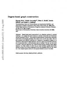
procedure main() { return A() + B() + C(); } procedure A() { return max(4, 7); } procedure B() { return max(4.5, 2.5); } procedure C() { return max(3, 1); }

(a) Example Program

main

A

main

B

C

A

B

max0

max

(b) Context-Insensitive

C

max1

(c) Context-Sensitive

Figure 1: Example Program and Call Graphs 2

Modelling Call Graphs

contour whose “local variables” correspond to the global variables of the program. Module scopes can be modeled similarly.

In the next subsection we present our general model of program call graphs in informal terms. We then formalize this model in lattice-theoretic terms.

2.1

Contours also represent lexical nesting relationships in the presence of lexically nested procedures. Each contour has a pointer to its lexically enclosing contour (which may be the global contour), except for the global contour which has no lexically enclosing contour.† In this fashion, we avoid losing precision during context-sensitive analysis of lexically nested procedures that access free variables.

Informal Model of Call Graphs

The program call graph is a directed graph that represents the calling relationships between the program’s procedures. * In a context-insensitive call graph, each procedure is represented by a single node in the graph. Each node has an indexed set of call sites, and each call site is the source of zero or more edges to other nodes, representing possible callees of that site; multiple callees at a single site are possible for a dynamically dispatched message send or an application of a computed function. Figure 1(b) shows the context-insensitive call graph corresponding to the example program in figure 1(a). In a context-sensitive analysis, a procedure may be analyzed separately for different calling contexts; each of these context-sensitive versions of a procedure is called a contour [Shivers 91b]. We model context-sensitive analyses in our call graph by having nodes in the call graph correspond to contours; thus, a call edge from a call site in one contour connects to the appropriate contour(s) of the callee procedure(s). The different context-sensitive analyses differ in how they determine what set of contours to create for a given procedure and which contours to select as targets of a given call. Figure 1(c) depicts one possible context-sensitive call graph for the same example program which distinguishes between calls to max with integer and floating point parameters. A context-insensitive analysis can be modeled by restricting the call graph to have only a single contour for each source-level procedure. We abstract these algorithm-specific decisions into a contour selection function which, given information about the call site’s calling contour and the possible classes of the actual parameters of the call, selects the set of callee contours to create (if not already present in the call graph) and link the call site to.

In languages with first-class function values or function pointers, we treat each such source-level occurrence of a function definition (or function whose address is taken) as creating a new class with a single method named apply whose body is the body of the function.‡ If the function was lexically nested within another function, then the class and its apply method are considered lexically nested in that same function. Evaluating the function definition or taking the address of a function are treated as instantiation sites of the new class, and invoking a function value is treated as sending the apply message to the object representing the function value. This encoding lets us focus solely on analyzing the flow of class instances through the program. We also need to record sets of possible classes for each instance variable, in a manner similar to class sets for local variables. To support array classes, we introduce a single instance variable per array class to model the elements of the array. To support both context-insensitive and -sensitive analyses of instance variable contents, each instance variable declaration is modeled by one or more instance variable contours. An instance variable contour maintains a single set of classes, representing the possible classes of values stored in that instance variable contour at run-time. Most analyses are context-insensitive with respect to instance variables, in that there is a single instance variable contour for each sourcelevel instance variable declaration. More precise analyses could maintain separate instance variable contours for each inheriting subclass, enabling the analysis to track the possible classes in each instance variable separately. We abstract these algorithm-specific decisions into an instance variable contour selection function

In addition to the set of callees at each call site, each contour in our call graph also records a set of classes for each formal parameter, local variable, and result of the procedure represented by the contour. These sets of classes represent the possible classes of values stored in the corresponding variables at run-time. To record the class sets for global variables, we introduce a special root *

†

Our model could be extend to support a lexically enclosing contour selection function that maps each contour to a set of lexically enclosing contours. This extension would allow us to model the flexible analysis of lexical environments supported by infinitary control flow analysis [Nielson & Nielson 97]. ‡ A similar strategy is used by the Pizza implementation to translate closures into Java [Odersky & Wadler 97].

We will use the terms procedure, function, and method interchangeably. Our system treats them uniformly.

2

GT Opt

Sound

G⊥

Gideal

This diagram depicts a lattice whose elements are call graphs. We order one call graph below another (and depict it in the cone below the other) if it is more conservative (less precise) than the other. The top and bottom elements, corresponding to the empty call graph and the complete call graph, respectively, are denoted by GT and G⊥. The point Gideal identifies the “real” but usually uncomputable call graph, which can be described precisely as the greatest lower bound over all call graphs corresponding to actual program executions. Any particular program execution induces a call graph in the cone above Gideal labeled Opt (for “optimistic”). Any call graph produced by a correct call graph construction algorithm must be in the cone below Gideal labeled Sound.

Figure 2: Regions in a Call Graph Lattice Domain

which returns the set of appropriate instance variable contours for a particular instance variable load or store operation, given class set information about the object being loaded or stored from.

2.2.1

The constructor Pow maps an input partial order D = 〈 S D, ≤ D〉 to a lattice DPS = 〈 SDPS, ≤ DPS〉 where SDPS is a subset of the powerset of SD defined as: S DPS = Bottoms(S) ∪

Some analyses are even more precise in their analysis of classes and instance variable contents. By treating different instantiation sites of a class as leading to distinct (analysis-time) classes with distinct instance variable contours, they can simulate the effect of templates or parameterized types without relying on explicit parameterization in the source program. We model these analyses by associating each source-level class with multiple class contours. A class contour selection function is applied at class instantiation sites to select the set of appropriate class contours to model the result of the instantiation. All previously described class information is generalized to be class contour information, including the sets associated with variables in each (procedure) contour, the actual parameter sets used by the (procedure) contour selection function and the instance variable contour selection function, and the information computed during the intraprocedural analysis of individual contours.

S ∈ PowerSet ( S D )

where Bottoms(S) = { d ∈ S ¬ ( ∃d' ∈ S, d'≤ D d ) }. The partial order ≤ DPS is defined in terms of ≤ D as follows: dps 1 ≤ DPS dps 2 ≡ ∀d 2 ∈ dps 2 , ∃d 1 ∈ dps 1 such that d 1 ≤ D d 2 If S1 and S2 are both elements of SDPS, then their greatest lower bound is Bottoms(S 1 ∪ S 2) . Each member of the family of constructors kTuple, ∀k ≥ 0, is the standard k-tuple constructor which takes k input partial orders D i = 〈 S i, ≤ i〉 , ∀i∈[1..k], and generates a new partial order T = 〈 S T, ≤ T〉 where ST is the cross product of the Si and ≤ T is defined in terms of the ≤ i pointwise, as follows:

To summarize, we use a single general model of the procedure call graph that can encode both context-sensitive and contextinsensitive call graphs. A wide range of context-sensitive call graphs can be represented by choosing different values for the three parameterizing functions: the contour selection function, the instance variable contour selection function, and the class contour selection function.

2.2

〈 d 11, …, d k1〉 ≤ T 〈 d 12, …, d k2〉 ≡ ∀i ∈ [ 1..k ] , d i1 ≤ i d i2

If the input partial orders are downward semilattices, then T is also a downward semilattice, where the greatest lower bound of two tuples is the tuple of the pointwise greatest lower bounds of their elements.

Lattice-Theoretic Model of Call Graphs

The constructor Map is a function constructor which takes as input an unordered set X and a partial order Y and generates a new partial order M = 〈 S M, ≤ M〉 where

This subsection formalizes the intuitive notions of the previous subsection using lattice-theoretic ideas.* This formalization ensures that we have a well-grounded understanding of contourbased call graphs and provides a vocabulary for discussing when a particular call graph is a safe (sound) approximation of the “real” call graph and when one call graph is more precise than another. We formalize the possible outputs of the contour selection functions, giving some formal structure to them that will help in comparing algorithms.

S M = { f ⊆ X × Y (x,y 1) ∈ f ∧ (x,y 2) ∈ f ⇒ y 1 = y 2 }

and the partial order ≤ M is defined in terms of ≤ Y as follows: m 1 ≤ M m 2 ≡ ∀(x,y 2) ∈ m 2 , ∃(x,y 1) ∈ m 1 such that y 1 ≤ Y y 2 If the partial order Y is a downward semilattice, then M is also a downward semilattice, where if m1 and m2 are both elements of SM, then their greatest lower bound is GLB 1 ∪ GLB 2 ∪ GLB 3 where: GLB 1 = { (x,y) (x,y 1) ∈ m 1, (x,y 2) ∈ m 2, y = glb(y 1, y 2) }

Figure 2 shows some of the interesting elements and regions in a call graph lattice. As is traditional in dataflow analysis [Kildall 73, Kam & Ullman 76] (but opposite to the conventions used in abstract interpretation [Cousot & Cousot 77]), the top lattice element represents the best possible (most optimistic) call graph, while the bottom element represents the worst possible (most conservative) call graph. *

Supporting Lattice Constructors

GLB 2 = { (x,y) (x,y) ∈ m 1, x ∉ dom(m 2) } GLB 3 = { (x,y) (x,y) ∈ m 2, x ∉ dom(m 1) }

A lattice D = 〈 S D, ≤ D〉 is a set of elements SD and an associated partial ordering ≤ DPS of those elements such that for every pair of elements the set contains both a unique least-upper-bound element and a unique greatest-lower-bound element. A downward semilattice is like a lattice but only greatest-lower-bounds are required. The set of possible call graphs for a particular model of context-sensitivity form a downward semilattice; we will use the term domain to refer to a downward semilattice.

Finally, the constructor AllTuples takes an input partial order D = 〈 S D, ≤ D〉 and generates a downward semilattice V = 〈 S V, ≤ V〉 by lifting the union of the k-tuple domains of D. Thus, the elements of SV are ⊥, all elements of 1Tuple(D), 2Tuple(D, D), 3Tuple(D, D, D) , etc., and the partial order ≤V is the union of the individual k-tuple partial orders with the partial order {(⊥,e)|e∈SV}.

3

ClassContour

= 2Tuple(Class, ClassKey)

ClassContourSet

= Pow(ClassContour)

InstVarContour

= 3Tuple(InstVariable, InstVarKey, ClassContourSet)

InstVarContourSet = Pow(InstVarContour) ProcContour

= 7Tuple(Procedure, ProcKey, ProcContour, Map(Variable, ClassContourSet), Map(CallSite, ProcContourSet), Map(LoadSite, InstVarContourSet), Map(StoreSite, InstVarContourSet))

ProcContourSet

= Pow(ProcContour)

CallGraph

= 2Tuple(ProcContourSet, InstVarContourSet)

Figure 3: Definition of Call Graph Domain 2.2.2

Call Graph Domain

in which the contour applies. The final component, ClassContourSet, represents the set of class contours stored in the instance variable contour. Similarly, the first two components of a procedure contour encode the source-level procedure declaration and the context to which this contour applies. The third component of the tuple, ProcContour, represents the lexically enclosing contour (if any) that should be used to analyze references to free variables. The fourth component maps each of the local variables and formal parameters of the contour’s procedure to a set of class contours representing the classes of values that may be stored in that variable. The variable mapping also contains an entry for the special token return which represents the set of class contours returned from the contour. The final three components of a procedure contour encode the inter-contour flow of data and control caused by procedure calls and instance variable loads and instance variable stores respectively.

We define call graphs in terms of three algorithm-specific parameter partial orders: ProcKey, InstVarKey, and ClassKey. The ProcKey parameter defines the space of possible contexts for context-sensitive analysis of functions, i.e., the output domain of the algorithm’s (procedure) contour selection function. The InstVarKey parameter defines the space of possible contexts for separately tracking the contents of instance variables, i.e., the output of the instance variable contour selection function. The ClassKey parameter defines the space of possible contexts for context-sensitive analysis of classes, i.e., the output of the algorithm’s class contour selection function. The ordering relation on these partial orders (and all derived domains) indicates the relative precision of the elements: one element is less than another if and only if it is less precise (more conservative) than the other. In addition to the three parameterizing partial orders, call graphs rely on several unordered sets that abstract various program features: Class is the set of source-level class declarations, InstVariable is the set of source-level instance variable declarations, Procedure is the set of source-level procedure declarations, Variable is the set of all program variable names, CallSite is the set of all program call sites, LoadSite is the set of source-level loads of instance variables, and StoreSite is the set of source-level stores to instance variables.

2.2.3

Soundness

A call graph is sound (i.e., safely approximates all possible program executions) if it is at least as conservative as each of the call graphs corresponding to possible program executions. Since the call graph domain is a downward semilattice, the greatest lower bound of all these program execution call graphs exists, and we notate it Gideal. Hence, a call graph G is sound iff it is equal to or more conservative than Gideal, i.e., G ≤cg G ideal . Unfortunately, in general it is impossible to compute Gideal directly, as there are in general an infinite number of possible program executions, so this observation does not make a constructive test for soundness of G.

Given the input parameter domains for a particular call graph construction algorithm and the sets abstracting program features, we construct the domain of call graphs, CG = 〈 S cg, ≤ cg〉, produced by that algorithm as shown in figure 3. The ProcContour and ProcContourSet definitions are mutually recursive; we intend these definitions to correspond to the smallest solution to these equations. Some of the context-sensitive algorithms introduce additional mutually recursive definitions that cause their CallGraph domains to be infinitely tall. To guarantee termination, at least one of their contour selection functions must incorporate a widening operation [Cousot & Cousot 77]. For example, Agesen’s Cartesian Product Algorithm uses elements of the ClassContour domain as a component of its ProcKey domain elements. In the presence of closures, this can lead to an infinitely tall call graph lattice; Agesen terms this problem recursive customization and describes several methods for detecting it and applying a widening operation [Agesen 96].

More constructively, a call graph is sound if, • for each procedure contour: • the (language-specific) intraprocedural dataflow constraints that relate the class contour sets of the contour’s variables (formals, locals, and the special result token) are satisfied, taking into account the result tokens of the callee contours at each call site and the contents of the accessed instance variable contours at each instance variable load site, • for each formal parameter of each callee contour at each call site, the formal’s class contour set is at least as conservative as the class contour set of the corresponding actual parameter at that call site,

The two components of a call graph are instance variable contours and procedure contours. Instance variable contours enable the analysis of dataflow through instance variable loads and stores. The first component, InstVariable, encodes the source level declaration that the contour is representing; the second component, InstVarKey, refines the first component by restricting the contexts

• for each instance variable contour accessed at each instance variable store site, the contents of the instance variable contour is at least as conservative as the class contour set of the value being stored at that store site,

4

Monotonic Refinement (moves down call graph lattice) Call Graph Unsound?

Initial Call Graph Construction

Call Graph Sound?

Select Step CallNext Graph

Final Call Graph

Additional Precision Desired? Non-Monotonic Improvement (moves up call graph lattice)

Figure 4: Generalized Call Graph Construction Algorithm 3.1

• and for each instance variable contour, the contents of the contour are at least as conservative as the contents of any instance variable contour with a less conservative key.

As described in section 2.2.2, the call graph lattice is parameterized over three domains, ProcKey, InstVarKey, and ClassKey, which together define algorithm-specific contextsensitivity. ProcKey is used as part of the algorithm’s procedure contour selection function: at each call site, for each applicable method, the selection function computes one or more elements of ProcKey that model the information about the call site that is relevant to the invoked method. For each procedure, the generalized algorithm maintains a table mapping ProcKey elements to their associated contours. By appropriately selecting ProcKey values, an algorithm indicates which call sites of a procedure should share contours and which should be given separate contours. When desired, the contour selection function may replace some existing contours with other contours, redirecting callers of the old contours appropriately. This may be done either to avoid producing too many contours for the method (by adding more general contours), or to increase the contextsensitivity in a portion of the analysis (by adding more specific contours). Similarly, InstVarKey models the possible outputs of the instance variable contour selection function, applied at each instance variable load and store site to model the relevant information at that site, and represents the ability of an algorithm to track the contents of a single source-level instance variable in multiple ways. Finally, ClassKey models some algorithms’ ability to distinguish different instances of a single class, primarily to track the contents of instance variables of the different class contours of a single class separately. At an instantiation site for class, an algorithm’s class contour selection function computes an element key of ClassKey to model the context of creation and downstream use, and the general framework uses the pair (class, key) as the class contour of the result of the instantiation. These various parameterizing domains are often interrelated, for example with different ClassKey elements giving rise to different ProcKey and InstVarKey elements to support specializing analysis of procedures and instance variables for different class contours.

The last constraint on instance variable contents ensures that different degrees of context-sensitivity for instance variables can coexist, while still ensuring that if a class contour is stored in an instance variable at one level of context-sensitivity, then it (or some more conservative class contour) appears in the contents of all more conservative views of that instance variable.

3

Contour Discrimination

Algorithmic Design Space

In this section, we present a generalized algorithm for call graph construction. The generalized algorithm is parameterized in several dimensions, and by selecting different values for the parameters it can express many previously described call graph construction algorithms. Figure 4 shows a schematic view of the generalized algorithm. The algorithm maintains a worklist of contours that are potentially unsound, initialized by the initial call graph construction process. The inner loop of the algorithm consists of evaluating the current call graph and selecting one of three possible actions: • If the current call graph is considered too imprecise (too far below Gideal in the lattice), the algorithm may apply NonMonotonic Improvement to improve the precision of the current call graph. • Otherwise, if the worklist is empty, the current call graph is sound and the algorithm terminates. • Otherwise, the algorithm applies Monotonic Refinement, removing a contour from the worklist and processing it to make it sound, thereby moving the resulting call graph one step closer to soundness and termination. The key parameters of the generalized algorithm are the choice of domains for ProcKey, InstVarKey, and ClassKey and the associated contour selection functions (section 3.1), the method used to construct the initial call graph (section 3.2), and the available nonmonotonic improvement operations, if any (section 3.4). Section 3.3 discusses monotonic refinement, which is the same in all algorithm instances. Section 3.5 contains a comparison of the relative precision of the call graphs produced by the various algorithms described in this section, and section 3.6 describes several aspects of our implementation of the generalized algorithm.

Typical values for these domains fall into several general categories: • single-point lattice: Selecting the single-point lattice (the lattice with only a ⊥ value) for ProcKey, InstVarKey, and ClassKey results in the degenerate case of a contextinsensitive analysis. Algorithms such as 0-CFA [Shivers 88, Shivers 91a], Palsberg and Schwartzbach’s basic algorithm [Palsberg & Schwartzbach 91], Hall and Kennedy’s

5

Table 1: Selected Algorithm Descriptions Algorithm

ProcKey

InstVarKey

ClassKey

0-CFA

single-point lattice

single-point lattice

single-point lattice

SCS

AllTuples(ClassContourSet)

single-point lattice

single-point lattice

b-CPA

AllTuples(ClassContour)

single-point lattice

single-point lattice

k-0-CFA where k>0

AllTuples(ProcContour)

single-point lattice

single-point lattice

k-l-CFA where k l > 0

AllTuples(ProcContour)

ClassContour

AllTuples(ProcContour)

call graph construction algorithm for Fortran [Hall & Kennedy 92], and Lakhotia’s algorithm for building a call graph in languages with higher-order functions [Lakhotia 93] are all examples of this instantiation of the framework. Algorithms that do not perform context-sensitive analysis of instance variables or classes use the single-point lattice for the InstVarKey or ClassKey domains, independently of their choice for the ProcKey domain.

• Contour keys in Agesen’s Cartesian Product Algorithm (CPA) [Agesen 95] are drawn from the domain AllTuples(ClassContour) , i.e., each key is a tuple of single class contours, one per formal parameter. At a call site, its contour selection function computes the cartesian product of the actual parameter class sets; a contour is selected/created for each element of the cartesian product. The “eager splitting” used as a component of each phase of Plevyak’s iterative refinement algorithm [Plevyak 96] is equivalent to this straightforward form of CPA.

• k levels of dynamic call chain: One of the most commonly used mechanisms for distinguishing contours is to use a vector of the k enclosing calling contours at each call site to select the target contour. If k = 0 , then this degenerates to the single-point lattice and a context-insensitive algorithm; k = 1 for ProcKey corresponds to analyzing a callee contour separately for each call site, and for ClassKey corresponds to treating each distinct instantiation site of a class as a separate class contour. An algorithm may use a fixed value of k throughout the program, as in Shivers’s k-CFA family of algorithms [Shivers 88, Shivers 91a] or Oxhøj’s 1-CFA extension to Palsberg and Schwartzbach’s algorithm [Oxhøj et al. 92]. Adaptive algorithms may use different levels of k in different regions of the call graph to more flexibly manage the trade-off between analysis time and precision. Finally, a number of algorithms based on unbounded but finite values for k have been proposed: Ryder’s call graph construction algorithm for Fortran 77 [Ryder 79], Callahan’s extension to Ryder’s work to support recursion [Callahan et al. 90], and Emami’s alias analysis algorithm for C [Emami et al. 94] all treat each non-recursive path through the call graph as creating a new context. Alt and Martin have developed an even more aggressive call graph construction algorithm, used in their PAG system, that first “unrolls” k levels of recursion [Alt & Martin 95]. Steensgaard developed an unboundedcall-chain algorithm that handles nested lexical environments by applying a widening operation to class sets of formal parameters at entries to recursive cycles in the call graph [Steensgaard 94]. For object-oriented programs, we define the k-l-CFA family of algorithms where k denotes the degree of context-sensitivity in the ProcKey domain and l denotes the degree of context-sensitivity in the ClassKey domain.

a

• In the worst case, CPA may require O(N ) contours to analyze a call site, where a is the number of arguments at the call site. To avoid requiring an unreasonably large number of contours, Agesen actually implements a variant of CPA that we term bounded-CPA (or b-CPA) that uses a single context-insensitive contour to analyze any call site at which the number of terms in the cartesian product of the actual class sets exceeds a threshold value. Our experiments suggest that only the bounded version of CPA scales beyond the realm of small benchmark programs. For example, on the instr sched benchmark (a 2,400 line Cecil program) b-CPA analysis completed in 146 seconds, while CPA analysis required 3,537 seconds. We observed similar slowdowns in the larger Java benchmarks (those over 10,000 lines). • A new algorithm, which we dub Simple Class Sets (SCS), draws its contour keys from the domain AllTuples(ClassContourSet) , i.e., each key is a tuple of sets of class contours, one per formal parameter. At a call site, its contour selection function simply selects a contour (possibly creating a new contour) whose key exactly matches the tuple of class sets that appear as actual parameters. If during re-analysis of a contour actual class sets at a call site change from their previous values, new contours are selected/created to exactly match the new actual parameters of the call. A bounded variant, b-SCS, could be defined to limit the number of contours created per procedure by falling back on a context-insensitive summary when the procedure’s contour creation budget is exceeded.

• parameter class sets: Another commonly used mechanism for distinguishing contours is to use some abstraction of the call site’s actual parameters. For example, some abstraction of the alias relationships among actual parameters has been used as the basis for context-sensitivity in algorithms for interprocedural alias analysis [Landi et al. 93, Wilson & Lam 95]. Similarly, several algorithms for interprocedural class analysis use information about the classes of actual parameters to drive their contour selection functions:

• In languages like Cecil [Chambers 93] and Strongtalk [Bracha & Griswold 93] which have expressive, but optional, parameterized static type declarations, using some abstraction of the static types of the actual type parameters to provide hints to the contour selection function may be very effective. • Finally, Pande’s algorithm for interprocedural class analysis in C++ [Pande & Ryder 94] is built upon

6

Landi’s alias analysis for C [Landi et al. 93] and uses an extension of Landi’s conditional points-to information as a basis for context-sensitivity.

associate a set of reachable classes and methods with each disjoint component [DeFouw et al. 97] (RTA pessimistically assumes that the dataflow graph only contains a single disjoint component, and thus computes a single set of reachable classes and methods for the entire program). Our algorithm for constructing Gunif is an adaptation of Steensgaard’s algorithm for near-lineartime points-to analysis of C programs [Steensgaard 96].

The CPA or SCS-style domains are also useful as InstVarKey domains, using the possible class(es) of the object whose instance variable is being accessed to select the right instance variable contour, tracking the contents of instance variables for different inheriting subclasses separately.

Since each of these flavors of G⊥ is sound and hence a legal solution, any of them would be a good initial call graph for algorithms that either do not wish to incur the expense of Monotonic Refinement to produce a sound call graph (which is true for all the algorithms listed above that start with some flavor of G⊥), or apply Non-Monotonic Improvement to improve the precision of the initially imprecise G⊥. The presence of first-class functions, however, may make call graphs close to G⊥ very imprecise, since each call site of such a function must be assumed to invoke any first-class function in the program with a matching number of arguments and static type signature. Of the above call graphs, only Gunif may reduce this problem.

• arbitrary: Plevyak’s “invokes graph” encodes an arbitrary mapping from each contour’s call sites to its callee contours [Plevyak 96]. It is clearly the most flexible of the mechanisms, but its lack of structure makes it difficult to easily explain or understand algorithms that rely upon it. Table 1 itemizes the domains chosen for ProcKey, InstVarKey, and ClassKey by the flow-sensitive algorithms that are experimentally assessed in section 4.

3.2

Possible Initial Call Graphs

Although it is possible to use any element of the call graph lattice domain as an initial call graph, all the algorithms of which we are aware start with one of two opposite extremes:

A potentially interesting new place to start call graph construction algorithms is Gprof, an optimistic call graph constructed from profile data from one or more runs of the program. Seeding the call graph with (context-insensitive) profile-derived call arcs and sets of classes can enable context-insensitive algorithms to reach the final sound solution more rapidly than if starting with GT, but without sacrificing precision. Profile data with call chain context [Grove et al. 95] can be used to seed some context-sensitive algorithms without degrading the final solution.

• GT: the top element of the call graph lattice. In practice, algorithms really begin with the call graph with only the global scope’s contour and the initial contour for the main function, with all variables in these contours mapped to empty class sets. This is the starting point used by the majority of the algorithms, including 0-CFA and k-CFA [Shivers 88, Shivers 91a], the Cartesian Product Algorithm (CPA) [Agesen 95], Plevyak’s iterative algorithm [Plevyak & Chien 94], and many others. GT is a good initial call graph for algorithms that apply Monotonic Refinement since it ensures reaching the best possible fixed-point solution for that algorithm.

3.3

Monotonic Refinement

Monotonic Refinement removes an unsound contour from the worklist and processes it, monotonically extending it (moving it lower in the contour domain) to make it locally sound. This involves performing intraprocedural class analysis of the contour beginning with the class sets of its formals, potentially adding to the class sets of local variables and adding new contours to call sites, load sites, and store sites. The centerpiece of this intraprocedural analysis is the analysis of message sends, which consists of the following steps:

• G⊥: the bottom element of the call graph lattice, i.e., the complete call graph with all call sites calling all contours and all variables holding all possible classes. In practice, a filtered version of G⊥ is used that has had some unnecessary call arcs and classes removed using statically available information or simple analysis: • Gselector: removes those call edges in G⊥ between call sites and contours with incompatible names or numbers of arguments.

1) The set of potentially invoked methods is computed by using the current class contour sets of the arguments to perform compile-time method lookup.

• Gstatic: uses the static types of variables and the type signatures of procedures to improve on Gselector by removing call arcs that are not statically type correct and removing elements from each variable’s class set that do not conform to the variable’s static type.

2) For each potentially invoked method, the algorithmspecific contour selection function selects and/or creates a set of contours for that method, called from this call site with these actual argument class contour sets, and these contours are bound to the call site in the calling contour. Any new contours created as part of contour selection are added to the worklist.

• Gintra: improves on either Gselector or Gstatic (depending on whether or not the language is statically typed) by performing intraprocedural analysis of each procedure to compute more precise approximations to the class sets of local variables and outgoing call arcs, as in Diwan’s Modula-3 optimizer [Diwan et al. 96].

3) The class contour sets of the actual parameters are added to the class contour sets of the corresponding formal parameters in each callee contour (using the ClassContourSet greatest-lower-bound operation to merge class contour sets). If any formal class contour set changes as a result, that callee contour is added to the worklist, since it may have become locally unsound and in need of reanalysis.

• GRTA: improves on Gstatic by performing Bacon and Sweeney’s Rapid Type Analysis (RTA), a linear-time optimistic reachability analysis, to eliminate classes that cannot be created and methods that cannot be invoked [Bacon & Sweeney 96]. RTA can be applied to dynamically typed languages as well to build a version of GRTA from Gselector.

4) Finally, the set of class contours returned from the message send is the greatest lower bound of the class contour sets bound to the return token in each callee contour.

• Gunif: improves on GRTA by performing a near-lineartime unification-based algorithm to identify disjoint components of the program’s dataflow graph and

Analysis of instance variable loads and stores is similar:

7

1) An algorithm-specific instance variable contour selection function selects and/or creates a set of instance variable contours for the instance variable being accessed (subject to the soundness restrictions discussed in section 2.2.3), typically based on the instance variable access site and the class contour set of the object being accessed. These contours are bound to the load or store site in the accessing contour.

call graph produced by starting from GT and applying monotonic refinement to completion. But the bottom-up strategy may produce acceptable results more quickly than the top-down strategy, can be interrupted at any time while still resulting in a sound solution, and may be a useful component in a program development environment where a sound but not necessarily optimal call graph is recomputed incrementally after each programming change.

2) For an instance variable store, the class contours for the value being stored are added to the contents class contour set of the accessed instance variable contours.

• Global Non-Monotonic Improvement is derived from Shivers’s proposal for reflow analysis [Shivers 91a]. Unlike local non-monotonic improvement it may examine large regions of the call graph during a single improvement step and may introduce new contours to the call graph. It occurs when an undesirable property of the current call graph is detected that cannot be corrected without making a jump from the current call graph to a (potentially unsound) call graph higher in the lattice. If this undesirable property is considered to be worth resolving, then the source of the imprecision is identified and additional contours are introduced at strategic points, in hopes of causing subsequent phases of Monotonic Refinement to rebuild the call graph without re-introducing the undesired imprecision.

3) For an instance variable load, the set of class contours returned by the load is the greatest lower bound of the contents class contour sets of the accessed instance variable contours. At class instantiation sites the class contour selection function generates a set of class contours, typically based on the sourcelevel class being instantiated and information from the current procedure contour. Analysis of variable references and assignments traverses the lexical contour links to locate the set of class contours associated with the accessed variable. For an assignment, the assigned class contour set is added to the variable’s associated class contour set, while for a reference the associated class contour set is returned as the result of the reference.

The only implemented algorithm of which we are aware that includes global non-monotonic improvement is Plevyak’s iterative algorithm [Plevyak & Chien 94]. The algorithm considers any message send with more than one possibly invoked method an undesirable property of the call graph and attempts to resolve it via non-monotonic improvement. Its control strategy computes a candidate sound call graph by running Monotonic Refinement to completion, followed by a check for Global Non-Monotonic Improvement. If refinement is desired, new contours are created and recorded in the “invokes graph” data structure for future reference in the contour selection functions. Then the algorithm iterates by resetting the call graph back to GT and reapplying Monotonic Refinement to completion to reach another candidate sound call graph. This overall process repeats until no more imprecisions can be resolved by introducing new contours, or too many iterations have been performed. One weakness of this coarse-grained control strategy is that large amounts of Monotonic Refinement analysis time may be spent reaching undesirable fixed-points. Our generalized algorithmic framework offers the possibility of intermingling Monotonic Refinement and Non-Monotonic Improvement on a much finer grain, perhaps reaching high-quality solutions faster.

Intraprocedural analysis of other kinds of statements and expressions in the method is language-specific but usually straightforward. Whenever a non-local set of class contours is read during intraprocedural analysis, including the result set of a callee contour, the contents set of an instance variable contour, or the set associated with a global or lexically enclosing variable, the generalized algorithm records a dependency link from the set to the reading contour. If the set later grows, the dependent reading contours are placed on the worklist, since the set of class contours upon which their intraprocedural analysis depended has changed.

3.4

Non-Monotonic Improvement

Each phase of Monotonic Refinement results in an output call graph that is lower in the lattice (more conservative) than its input call graph. In contrast, the output of each phase of Non-Monotonic Improvement is a call graph that is higher in the lattice than its input call graph. Algorithms for Non-Monotonic Improvement can be further classified informally as either Local or Global: • Local Non-Monotonic Improvement is characterized by a series of small, incremental steps up the call graph lattice. For example, the single intraprocedural “clean-up” pass performed to compute Gintra from Gselector or Gstatic can be viewed as one local non-monotonic improvement step per procedure. A further example of local non-monotonic improvement is based on the notion of exact unions. In a sound call graph, each variable’s class set must contain the class sets associated with all inflowing data flow arcs. However, algorithms starting from G⊥ often lead to class sets that are proper supersets of the union of their inflowing class sets. Such a call graph can be improved without making it unsound by replacing each variable’s class set with the exact union of its inflowing class sets. This narrowing may enable further downstream narrowings and removals of unreachable call arcs. This process continues until a fixed-point is reached. In the face of recursion, the call graph produced by starting from G⊥ and applying local non-monotonic improvement using exact unions to completion can be less precise than the

3.5

Relative Algorithmic Precision

Figure 5 depicts the relative precision of the final products of the various call graph construction algorithms described in sections 3.1 and 3.2 assuming that no procedure specialization is performed during compilation to preserve the contour-level view of the program (this matches the compilation configurations used during the experiments described in section 4). Algorithm A is depicted as being higher in the lattice than algorithm B if for all input programs GA is at least as precise as GB and there exists some program such that GA is more precise than GB. The k-l-CFA family of algorithms form an infinitely tall and infinitely wide sublattice. The k in the k-0-CFA, k-1-CFA, etc. subfamily of algorithms stands for an arbitrary, but finite value of k; infinite values for k are represented by the ∞-l-CFA family of algorithms (only ∞-0-CFA is shown). Under the no-specialization assumption, ∞-0-CFA, SCS, and CPA all produce call graphs with identical effective precision. Although the contours created by each of the three algorithms may be

8

GT Gprof1

Gprof2

Gprof3

Gprof4

Gprof5

…

Optimistic

…

Gideal

Sound … GSCS = GCPA = G∞-0-CFA

Gk-1-CFA …

…

…

Gk-0-CFA

G5-0-CFA

G4-1-CFA

G3-2-CFA

G4-0-CFA

G3-1-CFA

G2-2-CFA

G3-0-CFA

G2-1-CFA

G2-0-CFA

G1-1-CFA

…

G4-2-CFA

Gb-SCS

Gb-CPA

…

G5-1-CFA

G1-0-CFA G0-CFA Gunif(static) Gintra(static) Gintra(dynamic)

GRTA(static) Gstatic

Gunif(dynamic)

GRTA(dynamic)

Gselector G⊥

Figure 5: Relative Precision of Computed Call Graphs interprocedural analysis in the Vortex optimizing compiler infrastructure [Dean et al. 96] includes contour and contour_key abstract classes and related data structures, and a body of centralized code for executing the generalized algorithm and monotonic refinement. We are currently working on adding support for non-monotonic improvement. Instantiating the framework consists of implementing a concrete subclass of the ipca_algorithm class that implements the three contour selection functions. Abstract mix-in classes are provided that implement several of the common policies for managing procedure, instance variable, and class contours. The framework itself consists of approximately 4,000 lines of Cecil code and each of the instantiations measured in section 4 is implemented with 100-300 additional lines of code.

superficially quite different, if they are collapsed to reflect the lack of procedure specialization then all three call graphs will contain exactly the same call edges and class sets. However, the costs of computing each of the three call graphs are not the same. In the worst case, building the ∞-0-CFA call graph requires creating an infinite number of contours, building the SCS call graph requires creating an exponential number of contours, and building the CPA call graph requires creating a polynomial number of contours.* Despite its poor worst case behavior, the experimental results reported in section suggest that SCS may be the most efficient of the three algorithms.

3.6

Implementation

The generalized algorithmic framework is not only a useful tool for exploring the algorithmic design space and understanding previously described algorithms, but also leads to a flexible implementation framework. Our implementation of *

One of the most important considerations in the implementation of the framework was managing time/space tradeoffs. Most previous systems explicitly construct the entire interprocedural data and control flow graphs. Although this approach is viable for small programs, the memory requirements quickly become unreasonable during context-sensitive analysis of large programs. In our

We assume that the number of arguments to a procedure call is bounded by a constant, rather than being a function of program size.

9

implementation, we only explicitly store those sets of classes that are visible across contour boundaries (those corresponding to formal parameters, local variables, procedure return values, and instance variables). All derived class sets and all intra- and interprocedural data and control flow edges are (re)computed on demand. This greatly reduces the space requirements of the analysis, but increases computation time since dataflow relationships must be continually recalculated.

We performed our experiments on the suite of medium-sized Cecil and Java programs shown in Table 2. All experiments were performed on a Sun Ultra 1 model 170 with 256MB of memory.

Table 2: Benchmark Applications Program

Cecil Programs

We also found that the analysis time for the interprocedurally flowsensitive algorithms on the larger programs could be greatly reduced without a significant loss in precision by eagerly approximating class sets during set union operations. If the number of elements in the union exceeds a threshold value, then a compaction phase examines the elements to see if any classes already in the union share a common parent class. The candidate common parent that has the fewest number of subclasses not already included in the union is selected, and it and all of its subclasses are added to the union. This approximation reduces the size of the union (Vortex supports a compact “cone” representation for the class set corresponding to a class and all of its subclasses [Dean et al. 95]) and may reduce the number of times its contents change (by eagerly performing several subsequent class add operations). For example, for the three largest Cecil programs eager approximation reduced 0-CFA analysis time by a factor of 15 while only resulting in slowdowns of the resulting optimized executables of 2% to 8%.

4

Java Programs

Description

richards

400

Operating systems simulation

deltablue

650

Incremental constraint solver

instr sched typechecker new-tc compiler

Currently, the intraprocedural phase of interprocedural class analysis analyzes the entire procedure. We have recently implemented a sparse procedure representation that performs slicing to remove details of non-object data and control flow. Our initial experience has been that the sparse representation has little impact on Cecil programs (since virtually all dataflow is objectrelated), but that it reduced analysis time and memory usage by 50% for several of the smaller Java benchmarks. Unfortunately, our implementation is not yet complete and all the experiments in the section 4 utilize the old representation.

Linesa

2,400

Global instruction scheduler

20,000b

Typechecker for old Cecil type system

b

Typechecker for new Cecil type system

23,500

50,000

Old version of the Vortex optimizing compiler

toba

3,900

Java bytecode to C code translator

java-cup

7,800

Parser generator

espresso

13,800

Java source to bytecode translatorc

javac

25,550

Java source to bytecode translatorc

javadoc

28,950

Documentation generator for Java

a. Excluding standard libraries. All Cecil programs are compiled with an 11,000-line standard library. All Java programs include a 16,000-line standard library. b. The two Cecil typecheckers share approximately 15,000 lines of common support code, but the type checking algorithms themselves are completely separate and were written by different people. c. The two Java translators have no common code and were developed by different people.

Experimental Assessment 4.1

To determine how well different interprocedural analysis algorithms perform in practice, we implemented a half-dozen algorithm families using our framework and assessed them according to the following criteria:

Cost and Precision of Call Graph Construction Algorithms

An abstract comparison of the effectiveness of the algorithms can be made based on analysis time and space costs, and the precision of the resulting call graph. Table 3 reports, for each algorithm/ program pair, the analysis time in seconds, the growth in process size during analysis in MB*, the average number of contours per procedure, and the average number of times each procedure was analyzed. The difference of these last two numbers represents the average number of times per procedure that one of its contours was reanalyzed. For example, analysis of the instr sched program with the SCS algorithm took 83 seconds and the process size grew by 9.6 MB during analysis. On average, 6.5 contours were created for each procedure, each procedure was analyzed 8.5 times, and thus 2.0 contours per procedure were reanalyzed (and since analysis and re-analysis take roughly the same amount of time, approximately 25% of analysis time was spent reanalyzing contours)

• What are the relative precisions of the call graphs produced by the various algorithms? • What are the relative costs of the various algorithms, measured in terms of analysis time and memory space? • How do the differences in call graph precision translate into differences in effectiveness of client interprocedural analyses, in terms of program execution speed and executable size? The remainder of this section presents experimental results answering these questions for nine specific call graph construction algorithms: Gsimple (Gselector for Cecil, Gstatic for Java), RTA (extended to support first-class functions and multi-method dispatching), 0-CFA, b-CPA, SCS, and four instantiations of the kl-CFA family of algorithms. Section addresses the first two questions by presenting data on analysis time and space and call graph precision. Sections 4.2 and 4.3 address the remaining question: section 4.2 reports on the overall impact of interprocedural optimization and section 4.3 focuses on the individual contributions made by each of the interprocedural optimizations.

We see several trends in the data: *

10

This number only roughly approximates the actual maximum heap size during, and is sensitive to the heuristics used by the garbage collector to decide whether to launch a full collection or expand virtual memory.

Table 3: Analysis Time (secs), Heap Space (MB), Contours per Procedure, Analyses per Procedurea Gsimple

RTA

0-CFAb

SCS

b-CPA

1-0-CFA

1-1-CFA

2-2-CFA

3-3-CFA

richards

2 sec 1.6 MB 1.0 / 1.0

2 sec 1.6 MB 1.0 / 1.0

3 sec 1.6 MB 1.2 / 2.2

3 sec 1.6 MB 1.8/ 2.0

4 sec 1.6 MB 2.4 / 2.9

4 sec 1.6 MB 1.9 / 3.0

5 sec 1.6 MB 1.9 / 3.7

5 sec 1.6 MB 2.4/ 3.8

4 sec 1.6 MB 2.8 / 4.0

deltablue

2 sec 1.6 MB 1.0/ 1.0

2 sec 1.6 MB 1.0 / 1.0

5 sec 1.6 MB 1.4 / 2.4

7 sec 1.6 MB 3.75 / 4.25

8 sec 1.6 MB 4.8 / 5.7

6 sec 1.6 MB 2.5 / 4.0

6 sec 1.6 MB 2.5 / 4.0

8 sec 1.6 MB 3.6 / 6.1

10 sec 1.6 MB 5.0 / 8.2

instr sched

6 sec 2.5 MB 1.0 / 1.0

4 sec 2.5 MB 1.0 / 1.0

67 sec 5.7 MB 1.4 / 4.8

83 sec 9.6 MB 6.5 / 8.5

146 sec 14.8 MB 11.8 / 17.0

99 sec 9.6 MB 3.5 / 10.3

109 sec 9.6 MB 3.5 / 10.6

334 sec 9.6 MB 6.7 / 24.9

1,795 sec 21.0 MB 13.3 / 48.3

typechecker

26 sec 12.0 MB 1.0 / 1.0

25 sec 5.5 MB 1.0 / 1.0

947 sec 45.1 MB 1.2 / 4.6

13,254 sec 97.4 MB 8.7 / 31.4

new-tc

28 sec 6.9 MB 1.0 / 1.0

29 sec 6.9 MB 1.0 / 1.0

1,193 sec 62.1 MB 1.2 / 4.9

9,942 sec 115.4 MB 8.4 / 27.0

compiler

87 sec 0.2 MB 1.0 / 1.0

93 sec 22.4 MB 1.0 / 1.0

11,941 sec 202.1 MB 1.3 / 8.8

toba

35 sec 9.4 MB 1.0 / 1.0

18 sec 7.7 MB 1.0 / 1.0

79 sec 19.8 MB 1.0 / 1.0

67 sec 23.9 MB 1.1 /1.3

75 sec 19.8 MB 1.3 / 1.4

116 sec 20.3 MB 2.0 / 2.6

1,174 sec 19.8 MB 1.9 / 3.7

8,636 sec 19.8 MB 3.8 / 6.1

java-cup

80 sec 76.1 MB 1.0 / 1.0

89 sec 82.4 MB 1.0 / 1.0

116 sec 76.6 MB 1.0 / 1.2

112 sec 76.1 MB 1.2 / 1.5

124 sec 76.2 MB 1.4 / 1.6

145 sec 87.8 MB 2.2/ 3.1

2,086 sec 76.0 MB 2.1 / 5.7

espresso

49 sec 5.0 MB 1.0 / 1.0

74 sec 5.0 MB 1.0 / 1.0

136 sec 11.4 MB 1.0 / 1.4

307 sec 20.0 MB 1.8 / 2.5

305 sec 19.2 MB 2.0 / 2.9

1,183 sec 30.6 MB 3.7 / 7.3

51,646 sec 28.8 MB 3.6 / 16.3

javac

74 sec 27.6 MB 1.0 / 1.0

35 sec 27.4 MB 1.0 / 1.0

289 sec 27.4 MB 1.0 / 1.7

442 sec 27.8 MB 2.2 / 3.2

562 sec 27.5 MB 2.3 / 3.4

2,068 sec 60.1 MB 4.5 / 10.4

javadoc

66 sec 19.4 MB 1.0 / 1.0

38 sec 19.7 MB 1.0 / 1.0

169 sec 27.4 MB 1.0 / 1.3

165 sec 20.1 MB 1.6 / 1.9

208 sec 19.7 MB 1.6 / 2.0

295 sec 20.4 MB 2.6 / 3.6

27,991 sec 19.9 MB 2.1 / 5.9

a. Shaded cells correspond to configurations that either did not complete in 24 hours or exhausted available virtual memory (450MB). b. The average number of contours per procedure during 0-CFA analysis of Cecil programs is greater than 1.0 because procedures such as ‘if’ and ‘loop’ are analyzed with SCS contours. This limited context-sensitivity partially compensates for Cecil’s use of user-defined control structures.

abstractions such as sets and hash tables that are used by a number of clients. For the three larger Cecil programs 1-1CFA is infeasible, and for the compiler even 1-0-CFA fails to complete in under 24 hours.

• Analysis time for the flow-insensitive algorithms (Gsimple and RTA) appears to be roughly linear in the size of the program in practice (as well as asymptotically in the worst case); this suggests that they will scale gracefully to larger programs. In fact, running RTA in combination with the treeshaking optimization described in the next section usually results in a net reduction in compile time due to the removal of unreachable procedures.

• The SCS and b-CPA algorithms use different contour discrimination strategies to achieve approximately the same level of context-sensitivity. Although b-CPA has an asymptotically better worst case running time, for the programs in our benchmark suite SCS was uniformly faster.

• Increasing the value of k in the k-l-CFA algorithms for the two small Cecil programs does not result in a large increase of analysis time because most routines are only called from a small number of call sites (often only one). We start to see the expected exponential blow-up in analysis time in the slightly more realistic instr sched benchmark, which includes

• There is a much larger relative increase in analysis time between 1-0-CFA and 1-1-CFA for Java than there is for Cecil. This is due to a difference in the idioms used in the two languages. In Cecil, there is almost always just one textual occurrence of the object constructor for a class, within a user-

11

Table 4: Average Static/Dynamic Callee Procedures for call sitea Gsimple

RTA

0-CFA

SCS

b-CPA

1-0-CFA

1-1-CFA

2-2-CFA

3-3-CFA

richards

7.4 / 3.4

6.7 / 3.3

1.2 / 1.9

1.2 / 1.9

1.2 / 1.9

1.2 / 1.9

1.2 / 1.9

1.2 / 1.9

1.2 / 1.9

deltablue

10.2 / 8.1

9.4 / 7.3

1.4 / 2.2

1.4 / 2.2

1.4 / 2.2

1.4 / 2.2

1.4 / 2.2

1.4 / 2.2

1.4 / 2.1

instr sched

22.4 / 24.7

16.0 / 15.8

1.7 / 3.4

1.5 / 3.0

1.5 / 3.0

1.6 / 3.4

1.6 / 3.4

1.5 / 3.1

1.5 / 3.0

typechecker

46.7 / 59.3

42.9 / 53.4

4.4 / 13.9

4.0 / 11.9

new-tc

56.4 / 60.2

52.8 / 55.6

4.0 / 10.5

3.8 / 10.3

compiler

71.3 / 23.2

68.1 / 17.6

10.0 / 7.0

2.4 / 9.8

1.3 / 5.9

1.1 / 2.6

1.1 / 2.6

1.1 / 2.6

1.1 / 2.6

1.0 / 1.8

1.0 / 1.7

java-cup

3.2 / 10.9

2.2 / 6.9

1.1 / 2.6

1.1 / 2.6

1.1 / 2.6

1.1 / 2.6

1.0 / 2.1

espresso

2.2 / 10.8

2.1 / 10.1

1.7 / 9.7

1.7 / 9.7

1.7 / 9.7

1.7 / 9.7

1.6 / 8.7

javac

3.9 / 11.6

1.4 / 6.8

2.2 / 5.5

2.2 / 5.5

2.2 / 5.5

2.2 / 5.5

javadoc

3.1 / 11.1

1.4 / 7.2

1.2 / 3.4

1.2 / 3.4

1.2 / 3.4

1.2 / 3.4

toba

1.1 / 1.4

a. Shaded cells correspond to configurations that either did not complete in 24 hours or exhausted available virtual memory (450MB).

drive procedure specialization. However, because the Vortex compiler does not perform procedure specialization based on contours, summarizing the contour-level information to a procedure granularity will more accurately reflect the effective call graph precision seen by later stages of Vortex. Table 4 reports both the static and dynamic (computed by weighting each call site by its execution frequency in a sample program execution) number of callees per call site at a procedure-level granularity. We observe the following:

defined “constructor” method. In contrast, Java programs tend to use in-line object constructors (i.e. new expressions). Thus, there tends to be a much larger increase in the number of class contours under 1-1-CFA for Java than for Cecil. • The analysis times and memory requirements for performing the various interprocedurally flow-sensitive algorithms on the larger Cecil programs strongly suggest that the algorithms do not scale to realistically sized programs written in a language like Cecil. Scalability was better for the Java programs, but analysis times still were not linear in program size. It also appears that a large percentage of the analysis time is being consumed by contour reanalysis. We suspect that the majority of these reanalysis steps (especially for algorithms such as SCS and b-CPA that do not allow a contour’s incoming formal sets to be widened) are due to dependencies on the results of instance variable reads; when a new class is added to the contents of an instance variable, all accessing contours are reanalyzed. We are investigating seeding the instance variable contents with class sets derived from dynamic profile data for algorithms such as 0-CFA, SCS, b-CPA, and 1-0-CFA that perform context-insensitive analysis of instance variables. This may result in substantial reductions in contour reanalysis and thus overall analysis time, and make more sophisticated algorithms feasible on the larger Cecil programs. However, even if re-analysis time is sharply reduced, it appears that memory requirements may limit the scalability of the interprocedurally flow-sensitive algorithms.

• The interprocedurally flow-sensitive algorithms (0-CFA and above) produce call graphs that are substantially more precise than the simpler linear-time algorithms, but, for the benchmarks where analysis completed, the context-sensitive algorithms did not provide much additional precision over the context-insensitive 0-CFA algorithm. The RTA algorithm provides relatively small additional precision beyond Gsimple for the Cecil programs, but was more successful for the Java programs. The high degree of average polymorphism at call sites in Cecil programs under the flow-insensitive algorithms is mostly due to inaccuracy in modeling the flow of first-class functions. • In our benchmarks, the dynamic degree of polymorphism at call sites was usually higher than the static degree of polymorphism. Often the difference was quite large, which strongly suggests that purely static metrics may not accurately predict the impact on program execution speed. Based on this abstract precision data, we expect flow-sensitivity (0-CFA) to provide the main improvements in bottom-line execution speed, with flow-insensitive algorithms much worse and context-sensitive algorithms not much better.

Previous work has assessed the precision of call graph construction algorithms by reporting various metrics such as the average cardinality of class sets or the average number of callees at a call site in a contour. Although reporting these statistics at the granularity of contours can be useful for comparing various context-sensitive algorithms, it does not reflect the effective precision of the call graph unless multiple versions of each procedure are compiled, one for each of its analysis-time contours. Some previous systems [Cooper et al. 92, Plevyak & Chien 95] have used the contours created during interprocedural analysis to

4.2

Overall Impact

To assess the importance of call graph precision on the bottom-line performance impact of interprocedural optimizations, we compared, for each benchmark, the performance of a pair of base configurations that did not use interprocedural optimizations against pairs of configurations performing interprocedural

12

Java 1.25

4

1.00

3

0.75

Speedup

Speedup

Cecil 5

2

0.50

1

0.25

0.00

0 richards

base

deltablue

Gsimple

x + profile

instr sched typechecker

RTA

0CFA

tc2

compiler

SCS

b-CPA

toba

1-0CFA

java-cup espresso

1-1CFA

javac

2-2CFA

javadoc

3-3CFA

Figure 6: Application Execution Speed this information to more accurately estimate the potential effect of procedure calls on local dataflow information.

optimizations building on the call graphs produced by the different construction algorithms. • The base configuration represents an aggressive combination of intraprocedural and limited interprocedural optimizations which include: intraprocedural class analysis [Johnson 88, Chambers & Ungar 90], hard-wired class prediction for common messages (Cecil programs only) [Deutsch & Schiffman 84, Chambers & Ungar 89], splitting [Chambers & Ungar 89], class hierarchy analysis [Dean et al. 95], crossmodule inlining, static class prediction [Dean 96], closure optimizations (Cecil only), and a suite of traditional intraprocedural optimizations such as common subexpression elimination, constant propagation and folding, dead assignment elimination, and redundant load and store elimination. We applied these optimizations through our Vortex compiler to produce C code, which we then compiled with gcc -O2 to produce executable code.

• Exception detection: This interprocedural analysis identifies those procedures which are guaranteed to not raise exceptions during their execution. This information can be exploited both to streamline their calling conventions and to simplify the intraprocedural control flow downstream of calls to exception-free routines. • Escape analysis: Interprocedural escape analysis identifies first-class functions which are guaranteed not to out-live their lexically enclosing environment, thus enabling the function objects and their environments to be stack-allocated [Kranz 88]. This optimization applied only to the Cecil benchmarks. • Treeshaking: As a side-effect of constructing the call graph, the compiler identifies those procedures which are unreachable during any program execution. The compiler does not compile any unreachable procedures, often resulting in substantial reductions both in code size and compile time.

• The base+profile configuration augments base with profileguided class prediction [Hölzle & Ungar 94, Grove et al. 95]. • For each constructed call graph G, the base+IPG configuration augmented base with interprocedural analyses that enabled the intraprocedural optimizations in base to work better:

• The base+IPG+profile configuration augments the base+IPG configuration with profile-guided class prediction. We used the same dynamic profile data (derived from the base configuration) for all profile configurations. This methodology may slightly understate the benefits of profileguided class prediction in the base+IPG+profile configurations, but it eliminates an additional variable from our experiments.

• Class analysis: As a side-effect of constructing the call graph, each formal, local, global, and instance variable is associated with a set of classes whose instances may be stored in that variable. Intraprocedural class analysis exploits these sets as upper bounds that are more precise than “all possible classes,” enabling better optimization of dynamically dispatched messages.

Figure 6 displays application execution speed normalized to the speed of each application’s base configuration (raw data can be found in appendix A). The bars for the various profile configurations are shown behind the bars for the corresponding non-profile versions, highlighting any additional benefit from

• Mod analysis: This interprocedural analysis computes for each procedure a set of global variables and instance variables that may possibly be modified by calling the procedure. A number of intraprocedural analyses exploit

13

base+IPSCS that excluded class analysis was significantly slower than the version with all interprocedural optimizations enabled. The versions that excluded the other interprocedural optimizations showed slight decreases in execution time over the version with all optimizations enabled, but the differences were too small to be considered significant.

dynamic profile data in that configuration. Each pair of bars is labeled with the call graph construction algorithm used to produce the call graph used in that algorithm, or base for the noninterprocedural version. We draw the following conclusions from this data: • For most programs, the simple interprocedurally flowinsensitive algorithms, Gsimple and RTA, produced little improvement in execution speed, as foreshadowed by the high average degree of polymorphism at call sites shown in table 4.

Interprocedural escape analysis had little impact for the Cecil programs because the Vortex Cecil implementation allows programmers to annotate closures as LIFO (and thus nonescaping); virtually all of the closures in our benchmarks were annotated LIFO. When Vortex compiles ignoring these annotations, the modified base configurations run at half the speed of the base configurations used in this paper, but the base+IPSCS configurations run at essentially the same speed as reported previously. Thus, interprocedural escape analysis is sufficient to enable virtually all of the closure allocation optimizations enabled by the source level annotations. We chose to use the faster base configuration in the previous section to avoid overstating the benefits of interprocedural analysis; the cost of non-LIFO closures in the non-annotated base configuration could be somewhat reduced without resorting to interprocedural analysis by some simple intraprocedural techniques that Vortex does not implement due to the prevalence of LIFO annotations in the Cecil source code.

• For the Cecil programs, interprocedurally flow-sensitive algorithms (0-CFA and better) provided a significant boost in performance, with speeds ranging from 1.25 to 4.5 times faster. For the three smaller Cecil programs, interprocedurally flow-sensitive static analysis subsumed profile-guided class prediction, but profile data remained important for the larger Cecil programs. Context-sensitivity was less important, although it did have a measurable impact on the typechecker benchmark. This suggests that if it were feasible to apply context sensitive analysis to even larger Cecil programs, one might see additional benefit. • For the Java programs, interprocedural optimizations enabled modest improvements of between 0% and 13% over the base configuration. It should be emphasized that these speedups are relative to an already well-optimized base configuration; for comparison*, the base configuration is on average 7.6 times faster than Sun’s JDK1.0.2 interpreter, 3.8 times faster than Sun’s JDK1.0.2 just-in-time dynamic compiler, 2.0 times faster than Toba 1.0.5, an unoptimizing translator from Java to C, and 1.5 times faster than our own Vortex implementation [Dean et al. 96] without any optimizations other than those due to our gcc -O2 back-end.

5

In addition to the prior work studying particular algorithms for call graph construction already discussed in section 3, there exists a large body of prior work in interprocedural analysis and optimization. Typically this work has studied the impact of a single interprocedural analysis in the context of a single language. Closely related to ours is a trio of parameterized algorithms for interprocedural flow analysis of higher-order functional languages [Stefanescu & Zhou 94, Jagannathan & Weeks 95, Nielson & Nielson 97]. All three of these frameworks are similar to ours in that they support the construction of context-sensitive contourbased call graphs and are parameterized over ContourKeys, allowing them to express a variety of algorithms. Both Jagannathan & Weeks and Nielson & Nielson model formally the program’s semantics and treat interprocedural analysis as an abstract interpretation, while we formalize only the solution space of interprocedural analysis. All three frameworks are less general than ours in that they do not directly support non-monotonic improvement, initial call graphs other than GT, or object-oriented features such as message passing, or context-sensitive analysis of instance variable and class contours. We also extend their work by considering the issue of cross-algorithm precision comparisons and by implementing our framework in an optimizing compiler and assessing the impact of interprocedural analysis empirically. Additionally, the framework of Stefanescu and Zhou appears to be limited to only using various flavors of dynamic call chain information as contour keys. Agesen used templates as an informal explanatory device in his description of constraint-graph-based instantiations of 0-CFA, k-CFA, and Plevyak’s algorithm [Agesen 94]. Templates are similar to contours in that they serve to group and summarize all of the local constraints introduced by a procedure. Agesen does not formally define templates and only considers context-sensitivity in the ProcKey domain.

The treeshaking optimization shrank executable sizes for all the interprocedural analysis configurations. For the Java programs, executables were 10% to 20% smaller with treeshaking than the base configuration; the flow-sensitive algorithms typically reduced executable size by 0% to 3% more than the flowinsensitive algorithms. For the Cecil programs, decreases in executable size ranged from 15% on the compiler benchmark to 40% on the instr sched benchmark. Interprocedurally flowsensitive algorithms enabled reductions of an additional 10% over the flow-insensitive algorithms. Context-sensitive call graphs did not measurably improve the effectiveness of treeshaking on any of the benchmark programs.

4.3

Relative Value of the Interprocedural Analyses

The results presented in the previous section summarize the impact of a number of interprocedural analyses and optimizations into a single data point. Determining how much of the total speedup was attributable to each optimization would be useful in deciding which of the analyses would be most valuable to include in future compilers. To partially answer this question we built and measured several variations on the base+IPSCS configuration for the instr sched and javac benchmarks; each variation excluded one of the interprocedural analyses. By comparing the execution time of each variant against that of the full base+IPSCS configuration we can identify those analyses which have substantial performance impact. We found that virtually all of the improvement in execution speed was due to class analysis. The version of *

Other Related Work

Hölzle and Agesen compared the effectiveness of interprocedural class analysis based on the Cartesian Product Algorithm and profile-guided class prediction for the optimization of Self programs [Hölzle & Agesen 96]. They found that there was very little performance difference (less than 15%) between three optimizing configurations: one using only profile-guided class prediction, one using only interprocedural class analysis, and one

Our Java system does not currently implement null pointer dereference checks, multithreading, or dynamic class loading, so these comparisons to other Java implementations should only be used as evidence that our base configuration is efficient.

14

References

using both techniques. Our results for Cecil (a language similar to Self) differ in that flow-sensitive interprocedural class analysis alone appears significantly better than profile-guided class prediction alone.

6

[Agesen 94] Ole Agesen. Constraint-Based Type Inference and Parametric Polymorphism. In First International Static Analysis Symposium, September 1994. [Agesen 95] Ole Agesen. The Cartesian Product Algorithm: Simple and Precise Type Inference of Parametric Polymorphism. In Proceedings ECOOP ’95, Aarhus, Denmark, August 1995. Springer-Verlag.

Conclusions

We developed both a conceptual model and an implementation framework that encompasses a wide range of algorithms for call graph construction in object-oriented languages. Using this framework, we empirically assessed a variety of algorithms, applying them to a suite of medium-sized applications written in two different object-oriented languages. We found that interprocedural analyses, especially interprocedural class analysis, enabled substantial speedups for Cecil programs but only modest speedups for Java programs. In both languages, the additional precision of the call graphs constructed by the interprocedurally flow-sensitive algorithms had a large impact on the effectiveness of client interprocedural analyses and subsequent optimizations. However, the more precise contour-level call graphs constructed by the context-sensitive algorithms did not yield correspondingly large increases in application performance, in the absence of producing separate specialized compiled code for each procedure contour. Larger Cecil programs may benefit from contextsensitivity, but our experiments demonstrated that scalability problems prevent the context-sensitive algorithms from being applied beyond the domain of small benchmark programs. Thus the search for a scalable and effective call graph construction algorithm for programs that make heavy use of polymorphism and dynamic dispatching remains an open problem.

[Agesen 96] Ole Agesen. Concrete Type Inference: Delivering Object-Oriented Applications. PhD thesis, Stanford, January 1996. SLMI TR 96-52. [Alt & Martin 95] Martin Alt and Florian Martin. Generation of efficient interprocedural analyzers with PAG. In Proceedings of the Second International Symposium on Static Analysis, pages 33–50. Springer-Verlag, September 1995. [Bacon & Sweeney 96] David F. Bacon and Peter F. Sweeney. Fast Static Analysis of C++ Virtual Function Calls. In OOPSLA’96 Conference Proceedings, San Jose, CA, October 1996. [Bracha & Griswold 93] Gilad Bracha and David Griswold. Strongtalk: Typechecking Smalltalk in a Production Environment. In Proceedings OOPSLA ’93, pages 215–230, October 1993. Published as ACM SIGPLAN Notices, volume 28, number 10. [Callahan et al. 90] David Callahan, Alan Carle, Mary W. Hall, and Ken Kennedy. Constructing the Procedure Call Multigraph. IEEE Transactions on Software Engineering, 16(4):483–487, 1990. [Chambers & Ungar 89] Craig Chambers and David Ungar. Customization: Optimizing Compiler Technology for Self, A Dynamically-Typed Object-Oriented Programming Language. SIGPLAN Notices, 24(7):146–160, July 1989. In Proceedings of the ACM SIGPLAN ’89 Conference on Programming Language Design and Implementation.

We are hopeful that one of the new algorithmic instantiations presented in section 3, such as extensions of Gunif, local nonmonotonic improvement, or using Gprof as the initial call graph will result in an algorithm that offers both scalability and reasonable precision. Another important area of future work is investigating techniques to support incremental reconstruction of the program call graph and derived interprocedural information in the presence of program changes. Incremental algorithms would widen the applicability of interprocedural analysis by enabling it to be applied in new domains such as day-to-day program development and in environments that support dynamic class loading.

[Chambers & Ungar 90] Craig Chambers and David Ungar. Iterative Type Analysis and Extended Message Splitting: Optimizing Dynamically-Typed Object-Oriented Programs. SIGPLAN Notices, 25(6):150–164, June 1990. In Proceedings of the ACM SIGPLAN ’90 Conference on Programming Language Design and Implementation.

Acknowledgments

[Cousot & Cousot 77] Patrick Cousot and Radhia Cousot. Abstract Interpretation: A Unified Lattice Model for Static Analysis of Programs by Construction or Approximation of Fixpoints. In Conference Record of the Fourth ACM Symposium on Principles of Programming Languages, pages 238–252, Los Angeles, California, January 1977.

[Chambers 93] Craig Chambers. The Cecil Language: Specification and Rationale. Technical Report TR-93-03-05, Department of Computer Science and Engineering. University of Washington, March 1993. [Cooper et al. 92] Keith D. Cooper, Mary W. Hall, and Ken Kennedy. Procedure Cloning. In Proceedings of 1992 IEEE International Conference on Computer Languages, pages 96–105, Oakland, CA, April 1992.

Michael Ernst, Urs Hölzle, and the anonymous OOPSLA reviewers provided valuable feedback on earlier drafts of this paper. David Bacon encouraged us to develop the precision comparisons of context-sensitive algorithms depicted in figure 5. The use of exact unions during local non-monotonic improvement is due to Chris Colby. Finally, we wish to thank Bjarne Steensgaard for several helpful discussions of the area. This research is supported in part by an NSF grant (number CCR-9503741), an NSF Young Investigator Award (number CCR-9457767), a grant from the Office of Naval Research (contract number N00014-94-1-1136), an Intel Foundation Graduate Fellowship, and gifts from Sun Microsystems, IBM, Xerox PARC, Pure Software, and Edison Design Group.

[Dean 96] Jeffrey Dean. Whole Program Optimization of Object-Oriented Languages. PhD thesis, University of Washington, November 1996. TR-96-11-05. [Dean et al. 95] Jeffrey Dean, David Grove, and Craig Chambers. Optimization of Object-Oriented Programs Using Static Class Hierarchy Analysis. In Proceedings ECOOP ’95, Aarhus, Denmark, August 1995. Springer-Verlag. [Dean et al. 96] Jeffrey Dean, Greg DeFouw, Dave Grove, Vassily Litvinov, and Craig Chambers. Vortex: An Optimizing Compiler for Object-Oriented Languages. In OOPSLA’96 Conference Proceedings, San Jose, CA, October 1996.

15

[DeFouw et al. 97] Greg DeFouw, David Grove, and Craig Chambers. Fast Interprocedural Class Analysis. Technical Report TR-9707-02, Department of Computer Science and Engineering. University of Washington, July 1997.

guage Design and Implementation. [Nielson & Nielson 97] Flemming Nielson and Hanne Riis Nielson. Infinitary Control Flow Analysis: a Collecting Semantics for Closure Analysis. In Conference Record of POPL ’97: 24th ACM SIGPLAN-SIGACT Symposium on Principles of Programming Languages, pages 332–345, Paris, France, January 1997.

[Deutsch & Schiffman 84] L. Peter Deutsch and Allan M. Schiffman. Efficient Implementation of the Smalltalk-80 System. In Conference Record of the Eleventh Annual ACM Symposium on Principles of Programming Languages, pages 297–302, Salt Lake City, Utah, January 1984.

[Odersky & Wadler 97] Martin Odersky and Philip Wadler. Pizza into Java: Translating theory into practice. In Conference Record of POPL ’97: 24th ACM SIGPLAN-SIGACT Symposium on Principles of Programming Languages, pages 146–159, Paris, France, January 1997.

[Diwan et al. 96] Amer Diwan, Eliot Moss, and Kathryn McKinley. Simple and Effective Analysis of Statically-typed Object-Oriented Programs. In OOPSLA’96 Conference Proceedings, San Jose, CA, October 1996.

[Oxhøj et al. 92] Nicholas Oxhøj, Jens Palsberg, and Michael I. Schwartzbach. Making Type Inference Practical. In O. Lehrmann Madsen, editor, Proceedings ECOOP ’92, LNCS 615, pages 329–349, Utrecht, The Netherlands, June 1992. Springer-Verlag.

[Emami et al. 94] Maryam Emami, Rakesh Ghiya, and Laurie J. Hendren. Context-Sensitive Interprocedural Points-to Analysis in the Presence of Function Pointers. SIGPLAN Notices, 29(6):242–256, June 1994. In Proceedings of the ACM SIGPLAN ’94 Conference on Programming Language Design and Implementation. [Gosling et al. 96] James Gosling, Bill Joy, and Guy Steele. The Java Language Specification. Addison-Wesley, Reading, MA, 1996.

[Palsberg & Schwartzbach 91] Jens Palsberg and Michael I. Schwartzbach. Object-Oriented Type Inference. In Proceedings OOPSLA ’91, pages 146–161, November 1991. Published as ACM SIGPLAN Notices, volume 26, number 11.

[Grove et al. 95] David Grove, Jeffrey Dean, Charles Garrett, and Craig Chambers. Profile-Guided Receiver Class Prediction. In OOPSLA’95 Conference Proceedings, pages 108–123, Austin, TX, October 1995.

[Plevyak & Chien 94] John Plevyak and Andrew A. Chien. Precise Concrete Type Inference for Object-Oriented Languages. In Proceedings OOPSLA ’94, pages 324–340, Portland, OR, October 1994.

[Hall & Kennedy 92] Mary W. Hall and Ken Kennedy. Efficient Call Graph Analysis. ACM Letters on Programming Languages and Systems, 1(3):227–242, September 1992.

[Plevyak & Chien 95] John Plevyak and Andrew A. Chien. Type Directed Cloning for Object-Oriented Programs. In Proceedings of the Workshop for Languages and Compilers for Parallel Computing, pages 566–580, 1995.

[Hölzle & Agesen 96] Urs Hölzle and Ole Agesen. Dynamic vs. Static Optimization Techniques for Object-Oriented Languages. Theory and Practice of Object Systems, 1(3), 1996.

[Plevyak 96] John Plevyak. Optimization of Object-Oriented and Concurrent Programs. PhD thesis, University of Illinois at Urbana-Champaign, 1996.

[Hölzle & Ungar 94] Urs Hölzle and David Ungar. Optimizing Dynamically-Dispatched Calls with Run-Time Type Feedback. SIGPLAN Notices, 29(6):326–336, June 1994. In Proceedings of the ACM SIGPLAN ’94 Conference on Programming Language Design and Implementation.

[Ryder 79] Barbara Ryder. Constructing the Call Graph of a Program. IEEE Transactions on Software Engineering, 5(3):216– 225, 1979.

[Jagannathan & Weeks 95] Suresh Jagannathan and Stephen Weeks. A Unified Framework of Flow Analysis in HIgher-Order Languages. In Conference Record of POPL ’95: 22nd ACM SIGPLAN-SIGACT Symposium on Principles of Programming Languages, pages 393–407, January 1995.

[Shivers 88] Olin Shivers. Control-Flow Analysis in Scheme. SIGPLAN Notices, 23(7):164–174, July 1988. In Proceedings of the ACM SIGPLAN ’88 Conference on Programming Language Design and Implementation.

[Johnson 88] Ralph Johnson. TS: AN Optimizing Compiler for Smalltalk. In Proceedings OOPSLA ’88, pages 18–26, November 1988. Published as ACM SIGPLAN Notices, volume 23, number 11.

[Shivers 91a] Olin Shivers. Control-Flow Analysis of Higher-Order Languages. PhD thesis, Carnegie Mellon University, May 1991. CMU-CS-91-145. [Shivers 91b] Olin Shivers. Data Flow Analysis and Type Recovery in Scheme. In Topics in Advanced Language Implementation. MIT Press, 1991. Edited by Peter Lee.

[Kam & Ullman 76] John B. Kam and Jeffrey D. Ullman. Global data flow analysis and iterative algorithms. Journal of the ACM, 23(1):158–171, January 1976.

[Steensgaard 94] Bjarne Steensgaard. A Polyvariant Closure Analysis with Dynamic Abstraction. Unpublished manuscript, 1994.

[Kildall 73] Gary A. Kildall. A Unified Approach to Global Program Optimization. In Conference Record of the ACM Symposium on Principles of Programming Languages, pages 194– 206, Boston, Massachusetts, October 1973.

[Steensgaard 96] Bjarne Steensgaard. Points-to Analysis in Almost Linear Time. In Conference Record of POPL ’96: 23rd ACM SIGPLAN-SIGACT Symposium on Principles of Programming Languages, pages 32–41, St. Petersburg, Florida, January 1996.

[Kranz 88] David Kranz. ORBIT: An Optimizing Compiler for Scheme. PhD thesis, Yale University, February 1988. Department of Computer Science, Research Report 632.

[Stefanescu & Zhou 94] Dan Stefanescu and Yuli Zhou. An Equational Framework for the Flow Analysis of Higher-Order Functional Programs. In Proceedings of the ACM Symposium on Lisp and Functional Programming, pages 190–198, June 1994.

[Lakhotia 93] Arun Lakhotia. Constructing Call Multigraphs Using Dependence Graphs. In Conference Record of the Twentieth Annual ACM SIGPLAN-SIGACT Symposium on Principles of Programming Languages, pages 273–284, Charleston, South Carolina, January 1993.

[Wilson & Lam 95] Robert P. Wilson and Monica S. Lam. Efficient Context-Sensitive Pointer Analysis for C Programs. SIGPLAN Notices, pages 1–12, June 1995. In Proceedings of the ACM SIGPLAN ’95 Conference on Programming Language Design and Implementation.

[Landi et al. 93] William Landi, Barbara G. Ryder, and Sean Zhang. Interprocedural Side Effect Analysis With Pointer Aliasing. SIGPLAN Notices, 28(6):56–67, June 1993. In Proceedings of the ACM SIGPLAN ’93 Conference on Programming Lan-

16

Appendix A

Performance Data

The table below reports program execution times on a Sun Ultra 1 model 170 with 256MB of memory. Figure 6 is derived from this data.

Table 5: Execution Time (secs)

With Profile-Guided Receiver Class Prediction

Without Profile-Guided Receiver Class Prediction

Base

Gsimple

RTA

0-CFA

SCS

b-CPA

1-0CFA

1-1CFA

2-2CFA

3-3CFA

richards

0.14

0.13

0.12

0.10

0.10

0.10

0.10

0.10

0.10

0.10

deltablue

2.05

2.01

1.72

0.47

0.45

0.45

0.45

0.43

0.46

0.48

instr sched

1.09

1.03

1.14

0.52

0.49

0.49

0.51

0.54

0.52

0.49

typechecker

9.83

9.60

9.54

7.02

6.04

new-tc

9.68

9.20

9.57

6.94

6.80

compiler

193

195

195

155

toba

1.78

1.76

1.76

1.64

1.68

1.66

1.71

1.63

1.62

java-cup

0.22

0.21

0.21

0.21

0.21

0.21

0.21

0.21

espresso

1.76

1.65

1.65

1.65

1.55

1.57

1.69

1.68

javac

1.12

1.10

1.10

1.11

1.11

1.12

1.11

javadoc

1.23

1.21

1.21

1.23

1.20

1.24

1.22

1.20

richards

0.12

0.12

0.12

0.10

0.10

0.10

0.010

0.09

0.09

0.09

deltablue

0.71

0.58

0.57

0.45

0.43

0.42

0.44

0.43

0.44

0.44

instr sched

0.64

0.57

0.61

0.47

0.47

0.47

0.48

0.49

0.46

0.46

typechecker

6.65

6.72

6.83

5.80

5.61

new-tc

7.75

7.39

7.20

6.08

6.04

compiler

125

123

122

111

toba

1.76

1.75

1.75

1.63

1.66

1.65

1.67

1.63

1.61

java-cup

0.20

0.21

0.21

0.21

0.20

0.21

0.21

0.21

espresso

1.80

1.57

1.65

1.63

1.55

1.55

1.68

1.68

javac

1.11

1.08

1.09

1.12

1.09

1.09

1.10

javadoc

1.27

1.20

1.20

1.19

1.22

1.23

1.22

17

1.21