Property-Driven Dynamic Call Graph Exploration Michael Burch Eindhoven University of Technology Eindhoven
[email protected]
ABSTRACT
1
Analyzing and visualizing call relations can provide useful insights into the connectivities and linkings of certain parts of a software system. This can in particular be a good strategy to find software system parts that are interlinked a lot while others typically occur as more or less stand-alone components not called by many others. The challenging problem with call relation data comes from the dynamics of the data, i.e., a call graph can be changing either during the development of a software system or during the execution of the software. The second case mostly leads to long graph sequences changing on a fine-granular temporal scale requiring a suitable overview-based dynamic graph visualization technique. Moreover, identifying certain temporal patterns in the graph evolution can help to detect certain phases of either the evolution of a software system or phases during the execution that can show which components are connected while someone interacts with the runnable software for example. This can particularly based on graph, layout, or attribute properties, all providing different perspectives on the dynamics of the graph data. We illustrate the usefulness of our visualization technique by applying it to the open source software project JHotDraw. The call graphs are recorded during runtime while typical user interactions are applied.
Interacting with a software system at runtime may show if it works reliably or not, i.e., if problems like strange behaviors occur that are not easily fixable when inspecting the source code alone [16]. However, recording the call relations during runtime can help to identify functionality problems, but as a major challenge, such dynamic graph data can become temporally long involving hundreds or thousands of functions spread all over the software system hierarchy. For this reason an overview in form of a dynamic graph visualization is important to observe the time-varying call relation patterns and therefore, which calls may cause an erroneous functionality. Generally, dynamic graphs consist of at least three data dimensions that come in the form of vertices, edges, and time steps. Moreover, if the vertices are attached by an additional hierarchical organization, also this can be worth investigating. Edges may additionally carry weights and can be directed, finally, generating a dynamic network dataset. In particular, call relations in software systems belong to this special type of dynamic graph. The software entities like functions build the vertices that are related by calls, i.e., functions or methods call each other, building a call graph that can be changing over time. The functions typically build a level of granularity that can make the graphs rather big and hence, a hierarchical organization into subdirectories, directories, or packages may also be a useful concept in order to reduce the amount of graph vertices by filtering or by aggregating the call relations. This hierarchy aspect can be of particular interest, if the call relations have to be inspected on several hierarchical granularities. In this paper we introduce an algorithmic as well as visual approach to first, identify phases in dynamic call graphs and second, visualize those phases in a scalable dynamic graph visualization. The identification can be based on the graph topology, the hierarchical structure, or the visual properties given by the layout or vertex order implying link properties like link lengths or link orientations/directions. For the visual representation of the dynamic call graphs we use a time-to-space mapping, i.e., a mental map-preserving and scalable visualization technique based on the concept of interleaving introduced by Burch et al. [10]. Interaction techniques are integrated in the visualization tool while typical parameters influencing the visual appearance of the visualization can be changed on users’ demand. In this paper we add another list of interaction techniques based on the graph, hierarchy, and visual properties, but also those that explicitly exploit the computed phases to filter and navigate in the dynamic call graph data.
CCS CONCEPTS • Human-centered computing → Visualization techniques;
KEYWORDS Dynamic graph visualization, Software visualization, Edge splatting, Time-dependent data ACM Reference Format: Michael Burch. 2018. Property-Driven Dynamic Call Graph Exploration. In Proceedings of VINCI conference (VINCI’18), Jennifer B. Sartor, Theo D’Hondt, and Wolfgang De Meuter (Eds.). ACM, New York, NY, USA, Article 4, 8 pages. https://doi.org/10.475/ 123_4
Permission to make digital or hard copies of part or all of this work for personal or classroom use is granted without fee provided that copies are not made or distributed for profit or commercial advantage and that copies bear this notice and the full citation on the first page. Copyrights for third-party components of this work must be honored. For all other uses, contact the owner/author(s). VINCI’18, August 2018, Växjö, Sweden © 2018 Copyright held by the owner/author(s). ACM ISBN 123-4567-24-567/08/06. https://doi.org/10.475/123_4
INTRODUCTION
VINCI’18, August 2018, Växjö, Sweden We illustrate the usefulness of our technique by applying it to the open source software project JHotDraw in which the call relations are recorded during the runtime of the software system while a user interacts with the runnable software. This generates a dynamic call graph consisting of more than 1,000 directed and weighted graphs with several hundred hierarchically organized software entities and several thousand weighted call relations.
2
RELATED WORK
Dynamic call relations can be visually represented by means of dynamic graph visualization techniques [2, 3]. However, there are two camps of researchers, one focusing on graph animation and the others on static displays of dynamic graphs while the strengths and weaknesses of each of those are discussed controversially [28]. The first approach is denoted by time-to-space mappings while the second one is referred to as time-to-time mappings since the physical time is explicitly mapped to time in the visualization. These concepts are not only applicable to dynamic graphs, but also to several other time-varying datasets, e.g., time-dependent quantities [14]. In particular for call relations in software systems, Collberg et al. [15] introduced the Gevol tool that is based on nodelink diagrams and the fact that the individual time steps are displayed one after the other by keeping the graph layout stable, i.e., the nodes are placed at fixed positions preserving the mental map [24, 27]. Negatively, one cannot easily see different phases in the dynamic call graph since only one graph at a time is shown making it hard for comparison tasks due to our bad short term memory [20, 30]. In general, animations of dynamic graphs [17, 18] can make comparison tasks and the identification of certain phases problematic [1] which makes us apply a static time-to-space mapping to the dynamic call graph to better explore those phases over time. While depicting a graph sequence in a static way we can observe certain phases but negatively, if the graphs are rather dense and temporally long, those phases are difficult to identify visually. For this reason, we designed a visualization tool that supports the phase identification algorithmically based on typical call relation metrics like the call graph topology, the hierarchical organization of the software entities, or visual features given by the graph layout. We compute the number of relations over time either given by accumulated relation existences, relation weights, or relation densities, and plot those results to reflect a visual call relation distribution over time in a Cartesian representation [13] or a radial one [7] that also has some benefits [8]. This is similar to visually analyzing cluster evolution [25], but we additionally, provide a more aggregated overview first on several data and visual properties while allowing to compare the different phases based on certain metrics and visual features. Moreover, we provide a more graph comparison-based approach dividing all graphs into a set of categories based on Jaccard coefficient values for the graph edge sets. Burch et al. [9, 11, 12] describe a way to visualize dynamic graphs, in particular also dynamic call graphs, in a static
Michael Burch way, but negatively, in their approach the call relations are either abstracted to pixel-based graphical primitives or the provided views on the data do not scale to very long graph sequences. Their approach is not useful to automatically identify call relation phases. This is similar to the work of Burch et al. [13] in which a bipartite node-link diagram is used for the call relations that suffers from visual scalability problems, but positively a certain number of graphs can be visually compared to identify dynamic patterns without the explicit support by algorithmic concepts. The parallel edge splatting relies on interaction concepts that show the added and deleted edges over time, only globally, but not on different relation metrics or hierarchy properties. Also the concept of rapid serial visual presentation (RSVP) [4] has been investigated making the dynamic call graph visualization more scalable in the time dimension, but with the drawback of not providing a sufficient overview about the dynamics, i.e., the user has to scroll a lot to inspect dynamic graphs consisting of thousands of time steps. In a recent paper, Burch [6] added contour lines to the dynamic graph visualization helping to perceptually better identify the common and different visual patterns, but negatively, the viewers have to rely on their short term memory [20, 30] while comparing the individual abstracted patterns over time. This concept has been extended to allow comparisons of longer subsequences in a dynamic call graph by a call graph matrix [5] reducing the individual graph comparisons to real-valued numbers that are presented as a pixelmap. Although this approach reflects color coded density regions in the matrix supporting the identification of similarities and differences over time, it is not explicitly designed for identifying phases in dynamic call graphs nor on integrating call graph metrics and the hierarchical information. Also the visual properties of the given layout cannot be taken into account by this approach which is in focus of the current paper. To reach this goal we got inspired by the interleaved dynamic graph visualization that combines the massive sequence views [29] and the parallel edge splatting idea [13] with the goal to obtain a visual scalable visualization while still providing a perspective on the evolving graph structure.
3
DYNAMIC CALL GRAPH DATA
In this section we describe how static and dynamic call graphs can be modeled while the graph vertices are typically hierarchically organized in a software system hierarchy. Based on the dynamic graph data we explain how phases of call relations can be computed that can be based on the data only, but also on visual properties given by the graph layout or linear vertex ordering [19] if a bipartite layout is applied.
3.1
Static Call Graph
If there is no time-dependency involved in the call relations we refer this to as a static call graph reflecting a snapshot of the software system and its call relations between modules or software entities, i.e., packages, directories, subdirectories, files, or functions/methods depending on the hierarchical
Property-Driven Dynamic Call Graph Exploration granularity. A static call graph is mathematically modeled as 𝐺 = 𝑉, 𝐸 where 𝑉 := {𝑣1 , . . . , 𝑣𝑛 } denotes the finite set of vertices, i.e., in the specific case of a software system, it describes the software entities. The set 𝐸 := {𝑒1 , . . . , 𝑒𝑚 } ⊆ 𝑉 × 𝑉 denotes the finite set of directed edges, i.e., in the specific case of a software system, those express the call relations between software entity pairs. Moreover, if those call relations are weighted (for example by a time duration or a call frequency in a certain time interval) those weights can be expressed by an additional function 𝑤 : 𝐸 −→ R that maps each directed edge of the edge set 𝐸 to a real-valued number. It may be noted that certain weight functions may also require negative values depending on which metric is applied to a certain call relation.
3.2
Dynamic Call Graph
In the dynamic case we first compute all occurring vertices over time, i.e., we know all of the software entities in the evolution beforehand. Those can be built by generating a union set of all software entities in all time steps which finally, results in a union vertex set V denoting that all vertices between call relations might exist over time. The maximal possible edge set is given by E := V × V which would be the case if all software entities were connected by at least one relation over time, i.e., a scenario that will possibly never happen in a real-world scenario. But by this data model we can easily attach a time stamp to each edge which can be modeled by a time-varying function 𝑓 : E × N −→ R simply expressing that each edge between two vertices is mapped to a real-valued number at a discrete time point given by the natural numbers. This data model results in a dynamic weighted directed call graph, i.e., a dynamic call network.
3.3
Software System Hierarchy
Complementary to all vertices V in the union graph there exists a hierarchy 𝐻 = V∪𝑉𝐼 , 𝐸𝐼 that naturally structures all of the occurring software entities hierarchically. The new set of vertices consists of all of the vertices from the union graph plus those that are required for modeling the inner vertices expressed by the vertex set 𝑉𝐼 . The corresponding edge set in the hierarchy 𝐻 is modeled as 𝐸𝐼 ⊂ V ∪ 𝑉𝐼 × V ∪ 𝑉𝐼 expressing the parent-child relationships whereas 𝐸𝐼 ∩ E = ∅. Such a hierarchical information is useful to later compute certain call relation metrics like relations between vertices not leaving a certain subhierarchy level or relations between vertices located at a certain depth in a hierarchy. Moreover, the hierarchical organization may be used visually, for example, as data navigation aid or for collapsing and filtering out certain data elements.
VINCI’18, August 2018, Växjö, Sweden The goal of this work is to compute a subdivision of a dynamic call graph into a sequence of phases in which each phase reflects a dynamic property of the call relations. Consequently, the dynamic graph is split into a sequence of phases based on a property 𝑝 resulting in 𝑆𝑝 := 𝑃1 , . . . , 𝑃𝑛 in which each phase can have a different period length.
(a)
Phase Identification
A phase can be regarded as a closed period of time 𝑃 := 𝑡𝑘 , 𝑡𝑘+𝑖 indicated by a certain well-defined metric that is defined on each graph in a sequence separately. 𝑡𝑘 and 𝑡𝑘+𝑖 are fixed time steps indicating start and end points of a phase.
(c)
Figure 1: Illustrating the splatting effect of an interleaved dynamic call graph visualization: (a) The original graph sequence with color coded weights. (b) The weight and link information is used to compute a density field that is again color coded. (c) Contour lines are added to perceptually enhance the diagram. Such a phase subdivision can be based on several aspects in the data like individual call relations, call relation groups, or call relation groups with weights in a certain time interval for example. Moreover, more complex relation patterns can be computed based on the hierarchical structure, i.e., the depth of a call relation in a hierarchy, the hierarchy levels it spans, or the depth of the least common ancestor of the involved software entities in the software system hierarchy. These phases are then rather built based on topology-based aspects of the graph or based on the hierarchy. But as another phase computation metric we can use the visual representation, i.e., the graph layout and spatial arrangements of the vertices that result, for example, in different link lengths or orientations and directions. Those properties are also useful since they can be used as direct visual interactions inspired by brushing and linking concepts already successfully applied in parallel coordinates plots [22]. Moreover, as also used in this work, the dynamic graph visualization can make use of edge splatting leading to density fields, i.e., the densities of certain spatial regions can be exploited to identify phases during the evolution of call relations. To reach this goal, the time-varying density values can be categorized into value classes on which the phase separation algorithm is applied. This can be done in a hierarchical way by first starting with the lowest values and then iteratively split the phases into subphases.
4 3.4
(b)
DYNAMIC GRAPH VISUALIZATION
Since we deal with very long time-varying call graphs, a dynamic graph visualization is required that focuses on visual scalability in order to generate an overview about dynamic visual patterns. Those patterns are then useful to explore the call graph data if they can be remapped from the visualization to the dynamic data in a reliable way. Hence, we
VINCI’18, August 2018, Växjö, Sweden
Michael Burch
Figure 2: Phase bars: Attaching the results of the phase identification algorithm in form of a color coded bar chart aligned with the dynamic call graph visualization. The phase bars are selectable and further interactions can be applied. base our approach on the recently designed idea of interleaving bipartite layouts, each representing a single static call graph [10]. Based on that, interactions are applicable and identified phases can be easily attached to the dynamic graph visualization which is in focus of this work as a novel contribution.
4.1
Interleaving and Splatting
We first transform each call graph based on the union vertex set V into a bipartite layout and place each of them in this layout to a horizontal time axis. The bipartite layout requires a certain stripe width in which each graph is positioned. Then the graph sequence is moved together denoted by an interleaving concept resulting in a compressed dynamic graph visualization still reflecting dynamic patterns and still being visually scalable in vertex, edge, and time dimensions. To reduce the amount of visual clutter we additionally apply edge splatting [13], i.e., a density field is computed from the link information. These scalar values are then color coded to finally, visually reflect dynamic call graph patterns (see Figure 1). After splatting, the dynamic graph visualization is enhanced by contour lines. The order of the vertices in the bipartite layout is given by the software system hierarchy, i.e., the traversal of the hierarchy can be modified in each hierarchy level, but the overall hierarchical organization remains the same. Following this strategy generates a visually scalable dynamic call graph visualization focusing on dynamic pattern detection and in particular, on phase identification and visualization.
4.2
Phase Sequence Visualization
The sequence of phases is given in a separate view denoted by phase bars. Each bar represents a corresponding metric value of call relations existing at a certain point in time. We typically apply the link density function since it can give an overview about the number of links existing in a specific time interval or a time point. The density values naturally reflect the effect of graph density, but in our visualization reduced to a one-dimensional horizontal line. Applying filter functions based on the graph topology, the hierarchical organization, as well as the vertex positions or link lengths can have an impact on the phase bars. Consequently, if a temporally long dynamic call graph has to be explored the user can apply these different properties, filter for them, inspect the phase bars and hence, can visually identify the different call graph phases as well as the software system elements that caused those phases. Interactively
observing a dynamic call graph from different perspectives can lead to suitable insights about possible problems that occur during the execution of a program. Figure 2 illustrates a scenario in which a phase bar sequence is given by color coded bar charts. The similar density values are given by the differently color coded rectangles (connected bars of similar height). Those can be used to identify phases in the dynamic call graph. Then they can be used as means for applying further interaction techniques reducing the amount of call relations until the user finds insights in the dynamic call graph data.
4.3
Interactions
There are several interaction techniques integrated in the visualization tool. The most prominent ones given by the original dynamic graph visualization technique are already described in the work of Burch et al. [10] illustrating the novel idea of interleaving bipartite node-link layouts and then splatting them. In this paper we add another list of interaction techniques to the already existing ones. Those are more based on the phase identification that is applicable in three different ways, i.e., by the graph topology, by the hierarchical organization, as well as by the graph layout and vertex order/positions resulting in different link properties. Those might be explorable by brushing concepts known from parallel coordinates approaches for multivariate data [21–23] due to the fact that they look visually similar. ∙ Topology-based I: Only calls starting or ending at a certain software entity can be selected showing if a certain software entity caused wrong call relations. ∙ Topology-based II: Only calls between certain software entity groups can be selected indicating if a certain group is responsible for wrong calls. This feature can be applied stepwisely to isolate a wrong call relation. ∙ Hierarchy-based I: Only calls between a certain hierarchy level can be selected, i.e., for example if they share a least common ancestor in the hierarchy. This is useful if we know something about the subsystem in which something goes wrong. ∙ Hierarchy-based II: Only calls at a certain hierarchy depth can be selected which is suitable to inspect the call relations on different levels of hierarchical granularities. ∙ Link property-based I: Only calls with a certain link length can be selected indicating the distance between calls provided the hierarchy is used for laying out the software entities in the bipartite layout.
Property-Driven Dynamic Call Graph Exploration
VINCI’18, August 2018, Växjö, Sweden
Figure 3: An interleaved and splatted dynamic call graph visualization for a call graph dataset recorded during runtime of the JHotDraw project. The dataset contains 982 software entities, 32,259 call relations, and 1,077 call graphs. The diagram uses a stripe width of 30 pixels, is splatted 3 times, and represented in a topographic color scale. ∙ Link property-based II: Only calls with a certain link orientation/direction can be selected reflecting if a call relation is wrong in a certain direction which can be useful for functions calling each other one after the other exchangeably. There are many more interaction techniques worth investigating but the above list is just an illustrating example which powerful operations can be applied to the dynamic call graph data, i.e., data-driven but also visualization-driven ones. If phases are identified and visually represented in form of color coded bar charts aligned with the dynamic call graph visualization, those can also be used as interaction means. For example, a density-based filter is applicable reducing the amount of phases and resulting in certain interesting dynamic call graph properties worth investigating. ∙ Density selection: The call relations of a certain density can be highlighted to further inspect the corresponding software entities. ∙ Density filter: Call relations in a certain density interval can be filtered out which gives a better overview about the remaining ones. ∙ Find similar phases: By selecting one density region, all similar ones can be highlighted. This can be done for similar density values but also for similar temporal lengths. Similarity means the user sets two thresholds for density values and temporal lengths. ∙ Call relation count: The phase bars can also be computed without integrating the weights of the call relations or the densities. Just the pure relation coverage
information can be taken into account for generating the phase bars. ∙ Classing: The density values can be computed for each time point separately, typically resulting in strongly varying value sequences that are difficult to observe for phases. We support the subdivision of the individual values into value categories, also denoted by classing. ∙ Logarithmic densities: If the densities are varying in their magnitude, a logarithmic scale can be applied to reduce the size of the value gap.
5
APPLICATION EXAMPLE
In this section we apply the dynamic call graph visualization to dynamic call graph data from the JHotDraw project. We first present an overview about the entire dataset that consists of 982 vertices (software entities), 32,259 weighted and directed edges (call relations), and 1,077 time steps (time stamps during program execution). Then we describe the interaction techniques focusing on phase identification applied to different graph, hierarchy, and visualization properties. Figure 3 illustrates the dynamic call graph visualization for the entire dataset by interleaving and splatting the sequence of bipartite node-link diagrams. The vertex order at the vertical axis is derived from the hierarchical organization, i.e., the software entities are equidistantly placed to a vertical onedimensional line by preserving the hierarchical organization. It may be noted that the hierarchy might be traversed to achieve an even better attached call graph visualization, e.g., focusing on reducing link lengths as an aesthetic criterion [26], but this is not in focus of this work.
VINCI’18, August 2018, Växjö, Sweden
Michael Burch
Figure 4: Filter for the graph topology, i.e., for software entity groups and call relations in between can help to identify certain call relation phases that are only occurring in user-defined regions, i.e., software system parts.
(a)
(b)
Figure 5: Applying a hierarchy-based interaction to inspect the dynamic call graph on different hierarchical granularities: (a) Only call relations between software entities on the deepest hierarchical level are shown, i.e., where the least common ancestor is the parent vertex. (b) Only call relations between software entities on the second deepest level are shown, i.e., the least common ancestor is the grandparent vertex. Attached to the dynamic call graph visualization we can see the phase bars visualized below the dynamic graph visualization. The phase bars in Figure 3 are based on all call relations with weights and accumulated density values. We can see that the naive subdivision into density-based phases already reflects some details about the evolving call graph structure. For example, at the very beginning (left hand side) we can detect a sequence of thin green bars that occur in a similar way close to the right hand side. Looking into details about the dynamic call graph reveals that the dynamic patterns are not absolutely identical, but several calls and the overall structure of the call graph subsequences are very similar as also indicated by the corresponding interleaved dynamic graph visualization.
Although the overview about the entire dataset already provides some interesting dynamic call graph patterns we are more interested in looking into specific data properties based on the graph topology. For this reason we decide to first inspect the dynamic call graph for features corresponding to the two larger blocks in the center of the dynamic graph visualization. Hence, we apply a filter for exactly those software entity groups and obtain Figure 4. We can see that there are only those two temporally longer subgroups of software entities that are connected by calls (apart from some other shorter time spans before and after). This means, there is specific functionality connected by calls that was triggered by the user while he interacted with the corresponding functionality of the software. In this particular case the user has
Property-Driven Dynamic Call Graph Exploration
VINCI’18, August 2018, Växjö, Sweden
(a)
(b)
Figure 6: Visualization features can be in focus of interaction like link properties: (a) Filtering for call relations between software entities that are not farther away than 5 entities in the vertical direction. (b) Also link direction/orientations can be used for applying a filter like diagonal links from top left to bottom right.
Figure 7: Using the phase subdivision into phase bars to filter the dynamic call graph temporally. In this scenario, the user selected three different phases that can be explored further for graph topology, hierarchy, or visualization features.
drawn two graphical objects in JHotDraw which initiated exactly those calls. Those belong to the software entities contained in the subfigures subdirectory, i.e., many calls from outside functionality points to functions related to drawing something which is a natural behavior due to the fact that the user actually starts drawing something interactively. We can dig deeper in the dynamic call graph data by, for example, looking for calls that only happen between certain hierarchy levels. In this specific scenario we can go down to the deepest hierarchy level and inspect call relations between exactly those software entities. In Figure 5 (a) we can see a dynamic call graph visualization that only depicts this information. In Figure 5 (b) we also allow call relations between software entities that have a least common ancestor in the hierarchy that is one level higher than the one in Figure 5 (a). We can directly spot the difference and see that some more call relations occurred in scenario (b). If we inspect the dynamic graph visualization of the entire dynamic call graph dataset we can also ask about visual properties, i.e., properties directly implied by the layout of the software entities and their order on the vertical axis. But also for these kinds of interactions, our visualization tool provides a solution which is given in Figure 6. In scenario
(a) the user explicitly asked for call relations that do not go further away than 5 software entities in the vertical direction. This feature is useful to detect call relations between the same function, i.e., in a recursive call for example. We also filtered for that, revealing an empty dynamic graph visualization, i.e., no calls appear by this filter meaning in this particular interaction scenario with the tool, there seems to be no recursive call. In scenario (b) we looked for call relations of a certain direction, i.e., those that point from top to bottom in a diagonal fashion. This feature can be useful to see call relations in a specific direction. It may be noted that the interactions can also be combined, i.e., one might filter for graph topology features and then look for closest software entities given by the layout for example. There are many more insights that can be detected by inspecting the static representation of a dynamic call graph. The visualization is useful since it allows the user to freely look around and to search for patterns that can be compared with others while also looking at the phase identification charts. Moreover, by applying the specific interactions as well as the additional interaction techniques described in the work of Burch et al. [10] the visualization tool is equipped with a wealth of possibilities to explore dynamic call graph data. After the graph topology, hierarchy, or visualization properties are applied to subdivide the dynamic call graph into phases we can now use the phase bars as means for further interactions, i.e., to filter the dynamic call graph in the time dimension. Such a scenario is illustrated in Figure 7 in which a user selected three different phases that are worth investigating for further data explorations.
6
CONCLUSION AND FUTURE WORK
In this paper we described a dynamic call graph visualization technique that is visually scalable in the number of software entities, number of call relations, and the number of call graphs over time. Moreover, we described an approach to identify certain call relation phases based on the call graph topology and the hierarchical software system structure. Additionally, the layout and order of the software entities in the
VINCI’18, August 2018, Växjö, Sweden dynamic call graph visualization can be used to compute a number of relevant call relations based on the link properties like lengths and orientations. On top of that, time-varying density values of the link coverage can be computed that build the basis for subdividing the dynamic call graph into a sequence of phases. Those phases might be matched with specific interactions that someone applies during a running software system and can hence, be helpful to identify certain design flaws over time and software entities. Our dynamic call graph visualization tool is interactively useful as demonstrated in the application example involving a large dynamic call graph consisting of hundreds of software entities, thousands of call relations, and more than 1,000 time steps. For future work we plan to extend the visualization tool by further interaction techniques. Moreover, we should evaluate the visualization tool with real software engineers serving as experts in a corresponding user experiment. Since our dynamic graph visualization is visually scalable we might also combine software evolution and software execution by visually comparing dynamic call graphs during runtime for every revision during the evolution.
REFERENCES [1] Daniel Archambault, Helen C. Purchase, and Bruno Pinaud. 2011. Animation, Small Multiples, and the Effect of Mental Map Preservation in Dynamic Graphs. IEEE Transactions on Visualization and Computer Graphics 17, 4 (2011), 539–552. [2] Fabian Beck, Michael Burch, Stephan Diehl, and Daniel Weiskopf. 2014. The State of the Art in Visualizing Dynamic Graphs. In EuroVis - STARs. 83–103. [3] Fabian Beck, Michael Burch, Stephan Diehl, and Daniel Weiskopf. 2017. A Taxonomy and Survey of Dynamic Graph Visualization. Computer Graphics Forum 36, 1 (2017), 133–159. [4] Fabian Beck, Michael Burch, Corinna Vehlow, Stephan Diehl, and Daniel Weiskopf. 2012. Rapid Serial Visual Presentation in dynamic graph visualization. In Proceedings of the IEEE Symposium on Visual Languages and Human-Centric Computing (VL/HCC). 185–192. [5] Michael Burch. 2016. The Dynamic Call Graph Matrix. In Proceedings of the International Symposium on Visual Information Communication and Interaction (VINCI). 1–8. [6] Michael Burch. 2016. Isoline-Enhanced Dynamic Graph Visualization. In Proceedings of the International Conference on Information Visualisation (IV). 1–8. [7] Michael Burch, Fabian Beck, and Daniel Weiskopf. 2012. Radial Edge Splatting for Visualizing Dynamic Directed Graphs. In Proceedings of the International Conference on Computer Graphics Theory and Applications (IVAPP). 603–612. [8] Michael Burch, Felix Bott, Fabian Beck, and Stephan Diehl. 2008. Cartesian vs. Radial - A Comparative Evaluation of Two Visualization Tools. In Proceedings of the International Symposium on Advances in Visual Computing, ISVC. 151–160. [9] Michael Burch, Michael Fritz, Fabian Beck, and Stephan Diehl. 2010. TimeSpiderTrees: A Novel Visual Metaphor for Dynamic Compound Graphs. In Proceedings of the IEEE Symposium on Visual Languages and Human-Centric Computing, VL/HCC. 168–175. [10] Michael Burch, Marcel Hlawatsch, and Daniel Weiskopf. 2017. Visualizing a Sequence of a Thousand Graphs (Or Even More). Computer Graphics Forum (to appear) (2017). [11] Michael Burch, Christoph Müller, Guido Reina, Hansjörg Schmauder, Miriam Greis, and Daniel Weiskopf. 2012. Visualizing Dynamic Call Graphs. In Proceedings of the Vision, Modeling, and Visualization Workshop 2012. 207–214. [12] Michael Burch, Benjamin Schmidt, and Daniel Weiskopf. 2013. A Matrix-Based Visualization for Exploring Dynamic Compound Digraphs. In Proceedings of the International Conference on Information Visualisation, IV. 66–73.
Michael Burch [13] Michael Burch, Corinna Vehlow, Fabian Beck, Stephan Diehl, and Daniel Weiskopf. 2011. Parallel Edge Splatting for Scalable Dynamic Graph Visualization. IEEE Transactions on Visualization and Computer Graphics 17, 12 (2011), 2344–2353. [14] Michael Burch and Daniel Weiskopf. 2011. Visualizing Dynamic Quantitative Data in Hierarchies - TimeEdgeTrees: Attaching Dynamic Weights to Tree Edges. In IMAGAPP & IVAPP 2011 Proceedings of the International Conference on Imaging Theory and Applications and International Conference on Information Visualization Theory and Applications. 177–186. [15] Christian S. Collberg, Stephen G. Kobourov, Jasvir Nagra, Jacob Pitts, and Kevin Wampler. 2003. A System for Graph-Based Visualization of the Evolution of Software. In Proceedings ACM 2003 Symposium on Software Visualization. 77–86, 212–213. [16] Stephan Diehl. 2007. Software Visualization - Visualizing the Structure, Behaviour, and Evolution of Software. Springer. [17] Stephan Diehl and Carsten Görg. 2002. Graphs, They Are Changing. In Proceedings of the International Symposium on Graph Drawing. 23–31. [18] Yaniv Frishman and Ayellet Tal. 2004. Dynamic Drawing of Clustered Graphs. In Proceedings of the IEEE Symposium on Information Visualization (InfoVis). 191–198. [19] M. R. Garey and David S. Johnson. 1979. Computers and Intractability: A Guide to the Theory of NP-Completeness. W. H. Freeman. [20] Christopher G. Healey and James T. Enns. 2012. Attention and Visual Memory in Visualization and Computer Graphics. IEEE Transactions on Visualization and Computer Graphics 18, 7 (2012), 1170–1188. [21] Julian Heinrich and Daniel Weiskopf. 2009. Continuous Parallel Coordinates. IEEE Transactions on Visualization and Computer Graphics 15, 6 (2009), 1531–1538. [22] Julian Heinrich and Daniel Weiskopf. 2013. State of the Art of Parallel Coordinates. In Eurographics 2013 - State of the Art Reports, Girona, Spain, May 6-10, 2013. 95–116. [23] Alfred Inselberg and Bernard Dimsdale. 1990. Parallel Coordinates: A Tool for Visualizing Multi-dimensional Geometry. In IEEE Visualization. 361–378. https://doi.org/10.1109/VISUAL. 1990.146402 [24] Kazuo Misue, Peter Eades, Wei Lai, and Kozo Sugiyama. 1995. Layout Adjustment and the Mental Map. Journal of Visual Languages and Computing 6, 2 (1995), 183–210. [25] Sugeerth Murugesan, Kristofer Bouchard, Edward Chang, Max Dougherty, Bernd Hamann, and Gunther H Weber. 2016. Hierarchical Spatio-temporal Visual Analysis of Cluster Evolution in Electrocorticography Data. In Proceedings of the 7th ACM International Conference on Bioinformatics, Computational Biology, and Health Informatics. 630–639. [26] Helen C. Purchase, Robert F. Cohen, and Murray I. James. 1995. Validating Graph Drawing Aesthetics. In Proceedings of the International Symposium on Graph Drawing. 435–446. [27] H. C. Purchase, E. Hoggan, and C. Görg. 2007. How Important Is the “Mental Map”? – An Empirical Investigation of a Dynamic Graph Layout Algorithm. In Proceedings of the International Symposium on Graph Drawing. 184–195. [28] Barbara Tversky, Julie Bauer Morrison, and Mireille Bétrancourt. 2002. Animation: can it facilitate? International Journal of Human-Computer Studies 57, 4 (2002), 247–262. [29] Stef van den Elzen, Danny Holten, Jorik Blaas, and Jarke J. van Wijk. 2014. Dynamic Network Visualization with Extended Massive Sequence Views. IEEE Transactions on Visualization and Computer Graphics 20, 8 (2014), 1087–1099. [30] Colin Ware. 2004. Information Visualization: Perception for Design. Morgan Kaufmann Publishers Inc.