CALTECH ASCI TECHNICAL REPORT 105 cit-asci-tr105. Molecular dynamics simulations to compute the bulk response of amorphous. PMMA. S.B. Sane, T.
CALTECH ASCI TECHNICAL REPORT 105 cit-asci-tr105
Molecular dynamics simulations to compute the bulk response of amorphous PMMA S.B. Sane, T. Cagin, W.A. Goddard, W.G. Knauss
Molecular Dynamics Simulations to Compute the Bulk Response of Amorphous PMMA S.B. Sane * , T. Cagin** , W. A. Goddard** and W.G. Knauss* *
Graduate Aeronautical Laboratories, ** Material and Process Simulation Center California Institute of Technology, Pasadena, CA 91125, U.S.A.
Abstract The results of molecular dynamics computations and corresponding values of laboratory measurements are compared to assess the efficacy of the numerical method. Details are presented on the modeling process, including the selection of an appropriate force field derived from separate computations on isotactic (crystalline) PMMA together with commensurate experimental data. It is found that in addition to typical energy minimization and temperature annealing cycles to establish equilibrium models, it is advantageous to also subject the model samples to a cycle of a relatively large pressure excursion (GPa’s), to further improve the equilibrium state. Although the computations are limited to small samples in a physical sense (three polymer chains with fifty monomer units per chain per unit cell containing 2256 atoms), it appears that the primary limitation of the comparison with experimental data rests in the very short times (picoseconds). Estimates based on the time-temperature superposition principle do not overcome this difficulty, but may, on the other hand, signify limitations of the time-temperature tradeoff as normally practiced. 1. Introduction The increasing power of digital computational methods has offered the potential for “molecular dynamics” simulations to predict the mechanical properties of amorphous polymers. Molecular dynamics provides the possibility of determining basic physical properties that are difficult or laborious to access in the laboratory. However, this approach can become established as a laboratory substitute only after a large number of situations are studied both numerically and experimentally in comparisons. At present the
prediction of macroscopic properties using molecular models 1 is, at best, challenging and the question of the size of a numerical model for adequate property representation is of paramount concern. A number of studies have demonstrated the application of molecular simulation methods to compute (limited) mechanical properties of polymers (Fan and Hsu, 1992; Fan et al., 1994; Karasawa and Goddard, 1995), and results obtained from these simulations have been encouraging since they agree rather well with the laboratory measurements. However, in most of these cases the comparison between the experiments and the simulations were made at only one temperature, usually at room temperature. It is well known that in polymers the physical properties change substantially with time and temperature. Surprisingly little attention has being given to study the mechanical properties as a function of temperature using molecular dynamics simulation techniques. There have been a few efforts to study the relaxation behavior in polymers using molecular dynamics techniques (Fan et al., 1997). However, these investigations were concerned with mostly local and short time relaxation phenomenon through equilibrium MD. Long time chain relaxation processes are certainly beyond the scope of the conventional MD. Therefore, to explore complex properties such as uniaxial and shear response of the amorphous polymers requires treatment of these systems using nonequilibrium molecular dynamics techniques (Evans and Morriss, 1990; Gao and Weiner, 1996; Sarman et al., 1998). To data, most of the studies involving NEMD is on the short oligomers of Polyethylene (10-20 carbon atoms per chain) and focussed on obtaining shear viscosity as a function of strain rates (Khare et al., 1996; Lee and Cummings, 1998). Furthermore, the strain rates used in these studies were extremely high due to the time scales involved in the simulations. As a result of which the outcome from the simulations did not agree with the experiments. It would seem that determining bulk response (pressure-volume) should be one of the more readily successful computations for physical property determinations using equilibrium MD, because it deals typically with small macroscopic deformations and possesses a (mathematically) one-dimensional deformation character, unlike the case in shear or uniaxial deformations. Thus, the object of the present study is occasioned by
1
Simulated structures are composed of limited number of atoms.
non-trivial bulk compliance measurements that have become available on a real amorphous polymer system, Poly (Methyl-Methacrylate) (PMMA), which is also widely used in engineering and for utility items. Because such measurements are extremely difficult and time consuming, the computation alternative appears attractive. However, acceptance of molecular dynamics as a laboratory substitute hinges on the successful demonstration of complete equivalence in results derived from numerical methods, one must demonstrate that both the temperature and time controlled features of polymer behavior are correctly rendered. As a start one may deal with the time-independent range; however, that limitation needs to be narrowed in the future. The present computations are thus a valuable, initial model example for comparing molecular dynamics computations with experimental data. Consequently, we present here a comparison of such computations on bulk compliance as a function of temperature with laboratory measurements made on PMMA specimens, discussing, at the same time, the relation of these computations valid for only very short-times with the corresponding measurements acquired at much longer time scales. The paper is organized by first giving the details of the simulation techniques and sample preparation procedure in Section 2. This is followed by a presentation of the experimental results on an amorphous PMMA system (Sane and Knauss, 2000) and those of the simulations in Section 3. We then present a comparison between the molecular dynamics simulation results and the experimental results. A summary in Section 4 concludes the paper. 2. Simulation Details and Sample Preparation In this section we outline the simulation methodology. It includes first a selection of a proper force field to accurately describe various interactions of amorphous PMMA, following which the method of the model sample construction is delineated. Finally, details of the simulations are presented. 2.1
Selection of Proper Force Field
A main ingredient in MD calculations is the description of forces between atoms (neighbors/molecules) as their centers move relative to each other. This description is characterized by a force field, which can be considered for analytical purposes, to be a
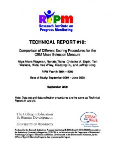
collection of energy terms characterizing interactions between atoms of a system. The potential energy, E, of a generic force field for an arbitrary geometry of molecules is typically characterized by the following terms: E = EB + EA + ET + EI + Evdw + EQ The first four terms represents bond interactions, namely, bond stretching (EB), bending (EA), torsion (ET ), and inversion (EI). The last two terms represents non-bond interactions, possessing van der Waals (EVdW) and electrostatic (EQ) character. Different functional forms may be used for these energy terms. The realism of the computation results hinges on the commensurate choice of the force field, i.e., on the proper expressions for the energy terms. A large number of force fields are available in the literature, optimized to represent different types of physical systems. To represent amorphous PMMA, the three most commonly used force fields were examined, namely, Universal Force Field (Rappé et al., 1992), Dreiding Force Field (Mayo et al., 1990) and COMPASS (Sun, 1998). In order to select the “best” force field from the three listed above, isotactic PMMA (iPMMA) was modeled. Isotactic PMMA is crystalline, yet a good structural analogue to amorphous PMMA, served, therefore, as an ideal structure for a force field evaluation because suitable properties obtained from X-ray structural analysis are available in the literature. The iPMMA crystals are orthorhombic with cell dimensions, a = 41.96 Å, b = 24.34 Å, and c (fiber axis) = 10.50 Å. Its molecular arrangement is represented by a double-stranded (10/1) helix (Kusanagi, et al., 1994). The model structure was assembled using the atomic coordinates illustrated in figure 1. The response of the iPMMA crystal structure was evaluated for different force fields by carrying out a full optimization of the atomic coordinates and cell parameters in comparison with the experimental data. To account for electrostatic interactions, the charges were derived from the QEq method (Rappé and Goddard, 1991). The PMMA monomer is shown in figure 2 along with the nomenclature used for the different atoms. The corresponding charges obtained from the
QEq method are shown in Table 1. Ewald summation was used for computing the nonbonded interactions. 2 Table 1: Charges (Coulomb) of different atoms in PMMA monomer unit. C1
-0.2411
C3
0.6862
H1C5
0.1888
H1C4
0.1321
C2
0.0213
O2
-0.5136
H2C5
0.0718
H2C4
0.1751
H1C1
0.1512
O1
-0.5877
H3C5
0.1677
H3C4
0.1197
H2C1
0.1087
C5
-0.0930
C4
-0.3872
The crystal structure was first subjected to multiple cycles of energy minimization, followed by a comparison between the experimental and the simulated crystal data under the three different force fields, as illustrated in Table 2. From that table one observes considerable disagreement between experiment and simulation for the universal force field and hence it was discarded from further consideration. The crystal structure was then subjected to NPT dynamics 3 at 300 K and at atmospheric pressure using the Dreiding and Compass force fields. A similar comparison between the experimental and simulated crystal data is presented in Table 3. Although the density of the simulated crystal structure was closer to the experimental value with the Compass force field, the cell parameters were in better agreement for the Dreiding force field, which indicated that the orthorhombic nature of the iPMMA crystal was better retained in the latter force field. Furthermore, the density of the crystal was (approximately) only 3% higher with the Dreiding force field, which implied that the Dreiding force field described the interactions in iPMMA in the best manner; it was, therefore, selected to represent the amorphous PMMA. The definitions of each of the energy terms for the Dreiding force fields used in the present study are listed in Appendix A. Van der Waal’s interactions are represented by the exponential 6-form as in the original paper (Mayo et al., 1990).
2
Ewald summation is a technique used for the calculation of non-bond interactions in periodic systems (Karawasa and Goddard, 1989). 3 NPT dynamics implies constant number of particles, pressure and temperature. For future reference, any XYZ dynamics implies constant X, Y and Z properties.
Table 2: Comparison of isotactic PMMA crystal data with experimental data after energy minimization. Cell Parameters Experimental data Universal force field Dreiding force field COMPASS force field
Density g/ cm3
a (Å)
b (Å)
c (Å)
α =β = γ
41.96
24.34
10.50
90o
1.210
44.31
23.66
11.06
90o
1.147
43.65
23.65
10.63
90o
1.210
43.88
24.05
10.29
90o
1.220
Table 3: Comparison of isotactic PMMA crystal data with experimental data after NPT dynamics. Cell Parameters Experimental data Dreiding force field COMPASS force field
2.2
Density g/ cm3
a (Å)
b (Å)
c (Å)
α
β
γ
41.96
24.34
10.50
90o
90o
90o
1.210
42.16
23.69
10.70
90.99o
90.36o
89.18o
1.245
46.29
24.63
10.51
89.32o
115.29o
89.81o
1.227
Amorphous PMMA Samples: Building and Optimization
Ideally computations extend over very large and very many molecules in suitably constructed interactive modes, so as to average the computations over a realistically large space domain. However, limitations of computer memory and speed still thwart such a general desire and one is forced to be satisfied with relatively small samples. To enlarge the spatial averaging scale one may, as a substitute, construct a (larger) number of sizefeasible molecule samples (models), and then average the response over these separate constructs with the expectation that they represent a reasonable average for a larger molecular model. In a trade-off between model construction time and statistical numbers of models, we chose to construct five distinctly different PMMA samples for averaging purposes.
All samples of amorphous PMMA contained 2256 atoms. Each one consisted of three polymer chains with fifty monomer units per chain. The bulk amorphous state was simulated by use of periodic boundary conditions; the polymer chains were packed into a unit cell and the cell was repeated in three dimensions. Each cell was therefore surrounded by 26 similar cells as nearest neighbors and if a portion of the chain exited the cell, it reentered the cell from the opposite surface. In effect, an infinitely periodic structure was created. Prior to building these samples, the charges shown in Table 1 were transferred to the monomer of PMMA. A typical sample of amorphous PMMA is shown in figure 3. The samples were constructed using the amorphous builder module available in Cerius2, a molecular modeling software program. 4 One of the important issues concerning amorphous polymers is the wide range of spatial conformations available to the polymer chains. These different possibilities were controlled, to some degree, via the two most important parameters affecting the sample configurations, namely, the backbone dihedral angles, which determines the orientation of different bonds with respect to each other, and the initial density which determines the chain packing in the unit cell. To construct PMMA samples as correctly as possible in a reasonable time frame, the polymer chains were generated by randomly assigning the backbone dihedral angles via the Monte Carlo method. 5 As demonstrated by Fan et al. (1994), random assignment of backbone dihedral angles followed by multiple cycles of energy minimization and molecular dynamics, produce similar results in generating polymer chains that are energetically as favorable as those obtained by the conventional method. 6 The initial density determines the packing of polymer chains in the unit cell and its neighbors, but restricts the conformational space spanned by each polymer chain. By specifying different initial densities and randomly assigning the backbone dihedral angles for each sample, the overall chain conformation attained in each sample is quite different.
4
Release 2.0, 1995, developed by Molecular Simulations Inc., 9685 Scranton Rd., San Diego, CA 921213752 5 Prior to energy minimization. 6 The conventional method for generation of polymer chains consists of a combination of the rotational isomeric state (RIS) model and the Monte Carlo method. However, this procedure is very time consuming.
The samples assembled in this manner were, therefore, judged to offer better statistically variant representations of the amorphous polymer. The densities specified were approximately 5 to 10% higher than the desired and experimental value of 1.18 g/cc at 300 K.7 These initial densities were achieved in three steps. Each sample was built starting at a density of approximately 0.8 g/cc. Lower density allowed the faster construction of the samples. The samples were then subjected to an energy minimization cycle. That was followed by a “temperature annealing cycle” involving NVT dynamics for a short duration (~ 5ps) at 600 K by keeping the cell dimensions fixed. Temperature annealing was necessary to prevent the system from getting trapped in a meta-stable, high-energy but “local” minimum. The sample density was increased by reducing the lengths of the unit cell and coupled with intermediate energy minimization at each step. This procedure was repeated until the initial target density was achieved for each sample. 8 Once the targeted initial density values were achieved, the samples were again subjected to energy minimization, with the cell parameters (a, b, c, α, β, γ) allowed to vary during this process. The initial and final values of densities for each sample are listed in Table 4. Ideally, the densities of the final structure should match the experimental values and be independent of their initial densities. However, due to the difference in the overall chain conformations of each sample and different initial densities, a variation in the final values of densities is observed. A comparison of the potential energies of each sample, also listed in Table 4, indicates similar values, which illustrates the effectiveness of the building procedure. The average value of the density obtained for the simulated structures is 1.16 g/cc with a standard deviation of 0.035 g/cc.
7
The initial densities specified are 5-10% higher than experimental density so that after performing full optimization, the final densities achieved for the samples are closer to the experimental density. 8 Prior experience with Polystyrene (PS) modeling, for which the target initial density was specified directly followed by energy minimization and temperature annealing cycles, revealed that if samples are not properly equilibrated during the building process, jumps in sample density may be observed while performing NPT dynamics. It could be especially true for the polymer chains with large side groups. Therefore, the method specified above was adopted for PMMA sample building.
Table 4: Initial densities, final densities, and potential energies of five PMMA samples at 0 K. Sample 1 2 3 4 5 average std. deviation
Initial Density (g/ cm3 ) 1.29 1.22 1.25 1.27 1.30
Final Density (g/ cm3 ) 1.189 1.133 1.169 1.117 1.198 1.162 0.035
Potential Energy (kcal/ mol) 10132.87 10085.96 10089.72 10188.72 10092.14 10117.88 43.92
The simulated structures must satisfy the criterion that the values of the internal stresses must be (close to) zero, which is equivalent to the structure being at a local minimum of the potential energy surface and assures thus an equilibrium state. The components of the internal stress tensor are defined as the first derivatives of the potential energy per unit volume with respect to strains.
σ ij =
1 ∂E V ∂ ε ij
where E is the potential energy, ε ij is the component of the strain tensor, and V is the volume of the system. The first derivative of the potential energy, the internal stress tensor at 0 K, with zero kinetic energy associated with atoms, is calculated by summing all forces acting between every pair of atoms.
σ
ij
=
1 2V
N
∑
k≠l
(r ik F jkl + r il F jlk ) =
1 2V
N
∑
(r ik − r il ) F jkl
k ≠l
where rik is the ith coordinate of atom k and Fjkl is the jth component of the interaction force between the kth and lth atoms. Table 5 shows the values of different stress components obtained by averaging over five the samples of PMMA. The values of the stress components clearly indicate that the polymer chains are mechanically relaxed. This criterion usually cannot be satisfied if the density of the simulated structure is fixed by not allowing the cell parameters to vary. The average cell parameters for the five
simulated structures are listed in Table 6. The deviations in cell lengths and angles are small even though full cell optimizations were performed. 9 Table 5: Average internal stress components (MPa) of five PMMA samples at 0 K. xx yy zz
0.367 ± 0.35
yz
0.178 ± 0.45
0.674 ± 0.73
xz
0.230 ± 0.25
0.912 ± 0.98
xy
0.244 ± 0.20
Table 6: Average cell parameters of five PMMA samples at 0 K. a (Å)
27.35 ± 0.52
α (degees)
89.98 ± 0.73
b (Å)
28.12 ± 0.75
β (degrees)
91.22 ± 1.86
c (Å)
27.98 ± 0.62
γ (degrees)
89.81 ± 2.42
The fundamental difference between a crystalline and an amorphous structure is the existence of long-range order in the former and its absence in the latter. The total pair distribution function, g(r), which gives a measure of the spatial organization of atoms about a central atom, can be used to demonstrate the long-range order in a structure. Therefore, the function g(r) can be utilized to distinguish between an amorphous and a crystalline structure. With this in mind, figure 4 (a) and (b) present g(r) for the simulated samples and isotactic PMMA crystals, respectively. The peaks of g(r) are an indication of presence of definite correlation between atoms within that radius. A comparison between figures 4 (a), which represents the amorphous structure, and (b), corresponding to the crystalline form, clearly demonstrates the difference in the nature of the two structures. The absence of any peaks beyond a 4 Å distance in figure 4 (a) indicates that there is no long-range order in the samples. The peaks observed at distances less than 4 Å can be assigned to the specific distances of closely coupled atoms. This spatial distribution function represents thus a completely randomized structure under the constraint on the cell size. In contrast, figure 4 (b) indicates the presence of peaks over much greater distances (approximately 8 Å), which implies the existence of a longer range order in the structure. 9
In addition to the atomic coordinates, the shape of the cell was free to change.
2.3
Simulation Details
Molecular dynamics simulations compute the motions of individual atoms in the system under the influence of the force fields and the surrounding environment. These motions are calculated via finite difference integration of the governing differential equations. One of the main objectives of equilibrium molecular dynamics is to determine the thermodynamic equilibrium properties of a system. If a microscopic dynamic variable, A, evolves in time as a function A(t), then the equilibrium value of A is computed by time averaging as shown in equation (1) (Haile, 1997). ∞
1 Aequi = lim ∫ A(t) dt T →∞ T 0
(1)
This dynamic variable can be any function of the atomic coordinates and momenta. Several forms of molecular dynamics are available, such as, NVT, NVE, etc. Appropriate forms of molecular dynamics need to be selected to compute the system properties of interest. The goal of the present study was to determine the bulk compressibility of PMMA as a function of temperature. This was achieved by computing pressure-volumetemperature (PVT) data using NPT dynamics. The bulk compressibility was then calculated from
KT = -
1 ∂v v∂P
or T
KT =
1 ∂ρ ρ ∂P
(2) T
The formulation of NPT dynamics was based on the work of Andersen (1980) and of Parrinello and Rahman (1980, 1981, and 1982). The Hoover method (1985) was used to specify the thermal coupling between the system and the heat bath; the thermal relaxation time, which dictates the coupling strength of the system to the heat bath, was set at 0.1 ps. The NPT molecular dynamics equations of motion dynamically control the system temperature and pressure at the specified values of external temperature and pressure. Thus the system was maintained under isobaric conditions with a specified
temperature. To accomplish this simulation, the cell dimensions represented by a matrix “h,” is introduced as a dynamical variable. To obtain a dynamical equation of motion for h variable, a “cell mass” parameter W is introduced, which may be viewed as representing the inertia of the system and determining the dynamic response of the system. Its value was chosen as 5% of the total mass of the atoms in the unit cell. This particular value was selected to ensure that the system equilibrates quickly and yields sufficient number of oscillations in volume during the course of simulation in order to obtain convergence in density and cell parameters without unnecessarily large fluctuations. The pressures considered were 0.0001 GPa (atmospheric pressure), 0.25, 0.5 and 1.0 GPa and the temperatures ranged from zero to 500 K, which encompasses the glass transition temperature of PMMA, Tg = 378 K. The simulations were carried out at the specified pressure starting at 100 K and progressively increasing the temperature to 500 K in 100 K increments. The duration of a typical dynamic run was for 25 ps with an integration time step ∆t of one femto-second. The first 10 ps of the simulations were approximately necessary to attain mechanical and thermal equilibrium; the final value of the density (or specific volume) at the specified pressure and temperature was obtained by averaging the density data over the remaining 15 ps. The system usually achieved equilibrium in first 5 ps; however, an additional 5 ps were allowed to ensure equilibrium in every case. Figure 5 shows the typical fluctuations in pressure, density and temperature data. One observes that the system quickly equilibrates in less than 5 ps and then continues to fluctuate around the equilibrium value. 3. Results and Discussion We next record the results obtained from experiments and from the simulations. We then present a comparison between the two data sets, which is followed by a discussion of the comparative study. 3.1
Results from Experiments
The dynamic bulk compliance of PMMA was determined at atmospheric pressure over a wide range of temperatures and frequencies. The measurements were carried out on irregularly shaped pellets ranging in weight from 0.1 to 0.3 gram, which were purchased
from ACE Company (ACE, now a part of Ono). The glass transition temperature was quoted by the manufacturer as 105 °C.10 The experimental technique used for measuring dynamic bulk compliance followed McKinney and Belcher’s work (McKinney and Belcher, 1963) and employed also in the more recent studies of Deng and Knauss (1997). It employs a small cavity in a (nearly) rigid solid containing the polymer specimen, a non-conductive, pressurizing fluid and two piezoelectric transducers, one serving as a volume expander and the other as a pressure sensor. A sinusoidal voltage applied to one transducer causes commensurate time-dependent pressure variations, which then interact with the second piezoelectric element (pressure sensor). The lengths of the stress waves associated with the applied frequencies are much larger than any of the cavity dimensions, so that the (volumetric) deformation of the sample in the cavity occurs under essentially quasi-static hydrostatic pressure. An experimental apparatus along with relevant electronic circuitry was developed in our laboratory by Deng and Knauss (1997). It served as the basic equipment for the measurements on PMMA with modifications in several aspects to make it suitable for measurements at suitable temperatures. For more details on the experimental setup and measurements, the reader is encouraged to refer to Sane and Knauss (2000). Here we present only a summary of the results. Measurements were made at temperatures between 27° to 123 °C on multiple samples and averaged for determining the dynamic bulk compliance. The storage and loss compliance over the frequency range of 10-1000 Hz is shown in figure 6. The measurements were quite repeatable for temperatures below 71 °C; however, uncertainties in the measurements increased up to ± 5 or 6% as temperatures approached the glass transition temperature. The maximum values of uncertainties were observed at high temperatures and low frequencies. The major transition of the storage compliance occurs at temperatures between 81° and 123 °C. Beyond 123 °C, PMMA is expected to approach the bulk rubbery domain. 11 At temperatures below 40 °C the bulk compliance changes more slowly with frequency than at the higher temperatures, and the loss compliance remains virtually constant; this represents the glassy domain. 10
Simulation computations of the glass transition temperature were also carried out. Appendix B provides more detail on this effort.
The experimental data was shifted using the time-temperature superposition principle to obtain a master curve, shown in figure 7, relative to 105 ºC. Both storage and loss compliance data were shifted by identical amounts. For later reference, the corresponding shift factors are shown in figure 8. It was observed that the bulk compliance data shifted well for temperatures below 92 ºC. However, beyond this temperature the curvatures of both the storage and loss compliance data did not match very well into a master curve, and it was therefore not reasonable to assign a degree of reliability to the shifted data in the high temperature range. 3.2
Simulation Results
To explore the effect of loading history on the bulk compressibility, two types of loading conditions were considered in the NPT dynamics simulations on the amorphous PMMA. In the first case, the external pressure was increased from 0.0001 to 1.0 GPa (loading conditions) and as a second case, pressure loading was decreased from 1.0 to 0.0001 GPa (unloading conditions) for each temperature. Simulations were carried out on the three samples and averaged. Figures 9 and 10 show the pressure variation of the density along an isotherm for loading and unloading conditions, and Table 7 lists the values of densities obtained at each pressure and temperature. From that table one gages the effect of loading history (loading vis-à-vis unloading) on the values of densities disappears at “high” pressures (approximately beyond 0.25 GPa), the difference in densities being generally less than 0.5%. However, near atmospheric pressures this difference is tangible. For example, at atmospheric pressure and 300 K, it is approximately 5%. More importantly, the slope of the isotherms, which according to equation 2 effect the bulk compressibility, are substantially different under loading and unloading conditions for lower pressures. Thus, to determine the bulk compressibility accurately at lower pressures, it is essential to determine the slopes of the isotherms carefully.
The current experimental set-up does not allow making reliable measurements beyond 123 ° C due to the beginning of thermal degradation of the pressure transmitting oil. 11
Table 7: Densities under loading and unloading conditions. Pressure GPa
Loading conditions
Unloading conditions
100 K 200 K 300 K 400 K 500 K 100 K 200 K 300 K 400 K 500 K
0.0001
1.144
1.133
1.109
1.098
1.098
1.196
1.177
1.161
1.149
1.144
0.2500
1.231
1.222
1.218
1.204
1.194
1.233
1.221
1.206
1.196
1.192
0.5000
1.274
1.268
1.256
1.246
1.237
1.271
1.265
1.251
1.243
1.240
1.0000
1.343
1.337
1.333
1.322
1.310
1.340
1.327
1.328
1.323
1.303
The differences in the densities and the slopes of the isotherms near atmospheric pressures (loading vis-à-vis unloading) is probably a feature of the modeling process rather than a physical phenomenon exemplifying permanent compressibility or yielding. To explore this model-conditioned behavior further, each model sample was first subjected to the loading cycle followed by an unloading cycle. After passing through this loading cycle, the polymer chains in the samples did not regain their original configurations and resulted essentially in squeezing out the excess volume present in the samples. The thermal cycling of the samples (i.e., going from zero to 500 K and back to zero K) further augmented the configurational changes in the samples; the polymer chains were able to sample different conformational spaces, which led to different local energy minima. From Table 8, one observes that there is a better agreement of the properties such as density and coefficient of thermal expansion between the experimental measurements and the results obtained from unloading case than as compared with the loading case. Furthermore, when the samples were loaded again (i.e., pressure increased from 0.0001 to 1.0 GPa) after being subjected to a complete loading-unloading cycle, the variation of density with pressure for each temperature followed almost the same path as obtained during the previous unloading conditions (the difference in densities obtained from unloading and reloading was less than 1%) as demonstrated in figure 11 for a particular case of 300 K. Thus one can infer that the initial loading (from 0.0001 to 1.0 GPa) of the samples should be considered as a part of sample conditioning (equilibration) process similar to temperature annealing cycles as mentioned in Section 2.
Table 8: Comparison of properties (density and coefficient of thermal expansion) at atmospheric pressure and 300 K between experimental results and those obtained under loading and unloading cases for amorphous PMMA. Coefficient of thermal expansion /K Density (g/cc) Below Tg
Above Tg
Experiments*
1.18
2.53 x 10⁻⁴
5.74 x 10⁻⁴
loading
1.11
1.00 x 10⁻⁴
3.00 x 10⁻⁵
unloading
1.16
1.00 x 10⁻⁴
3.00 x 10⁻⁴
*Experimental results were taken from Polymer Handbook (1989). Average values of PMMA were considered for comparison. In this context a comment is in order with respect to the sample conditioning during the construction phase. Recall that a part of the building process consisted of consolidation following an initial choice of the density. The pressurization histories described in this section provide, in principle, the same effect, except that larger consolidation pressures are incurred than those employed initially. This observation demonstrates clearly that the initial building process was insufficient to establish an energy-minimized equilibrium structure, but that higher pressure excursions are needed than might normally be surmised to arrive at an equilibrium model. With this understanding, we limit evaluations of the NPT data to the unloading portion of the pressure histories. Based on the set of pressure-density-temperature data as obtained from the unloading histories, the isothermal bulk compliance of PMMA was calculated as a function of temperature using equation 2. To compare the simulation results, excerpts from the laboratory measurements were selected as a function of temperature and at the single frequency of one kHz. That comparison between the simulations and the experimental results is shown in figure 12. Tables 9 and 10 list the bulk compliance values obtained from the computations and the measurements at one kHz at different temperatures. In figure 12 we have also included the bulk compressibility as computed from the PVT data for the initial loading conditions. The difference in the bulk compliance values obtained from this initial loading and from the unloading history
amounts to approximately a factor of two. In view of the fact that the magnitude of the bulk compliance changes by only a small factor of two or three throughout the viscoelastic transition, this difference in the computed bulk compliance is substantial and it appears, therefore, essential to condition the samples through a loading cycle prior to performing any computations.
Table 9: Bulk compliance (GPa)-1, as a function of temperature from the simulations at atmospheric pressure. Temperature (K)
Loading condition
Unloading condition
100
0.371
0.130
200
0.416
0.172
300
0.443
0.168
400
0.462
0.173
500
0.478
0.194
Table 10: Bulk compliance (GPa)-1, as a function of temperature from the experimental results at 1 kHz at atmospheric pressure. Temperature (K)
Bulk compliance at 1 kHz
300.54
0.169
311.71
0.169
322.40
0.184
333.34
0.183
344.15
0.199
354.88
0.244
365.20
0.257
375.54
0.287
385.96
0.292
396.01
0.311
Discounting the unreasonable effects derived from the initial loading history, the computations demonstrate the correct order of magnitude for the bulk compliance. However, the variation of the bulk compliance observed in the experimental data with temperature is much more pronounced than the computations indicate. This was expected because the computations provide information on the bulk behavior at very high frequencies on the order of giga hertz (or very small time scales on the order of nanoseconds) and only a small variation in the bulk compliance was observed over a temperature range of 100 to 500 K. In the full documentation of the measurements Sane and Knauss (2000) make a plausible argument, based on the (tentative) use of the timetemperature superposition principle, that the variation of the simulated compliance should not be significant over the temperature range considered. In contrast, the measurements reveal significant variations of the compliance of PMMA in the frequency range of 101000 Hz (in the milli-seconds time scale), and therefore over this frequency range the “glass-to-rubber” transition was observed a temperature range of 300 to 430 K. Another important issue deserving attention regards the modeling of the bulk compliance. It is often believed that the molecular mechanisms controlling bulk deformations depend only on very local motions of the polymer molecules and that long range entanglements (and cross-links) play no or a subsidiary role. In contrast, the shear behavior is supposed to be governed by local as well as long range molecular interactions and rearrangements. Therefore, it was believed that due of the presence of dominant local interactions in bulk behavior, predicting the bulk behavior for polymers using molecular modeling techniques would be relatively simpler and more accurate than predicting the shear behavior. However, in figure 8, the master curves corresponding of the bulk response data illustrate that the range of the bulk transition is extended over about eight decades of time or frequency, which is comparable to the transition range of the shear response (Sane and Knauss, 2000), which indicates that the molecular mechanisms controlling the bulk deformations may not just involve very local interactions. It has been suggested that the molecular contributions to the bulk deformations in PMMA could be derived primarily from the motion of the ester side groups, which are relatively massive, coupled with the motion of the chain backbone, with, however, the rotations and oscillations of the side groups playing a dominant role. These molecular
motions governing the bulk response are still relatively short-ranged as compared to medium and long-range interactions present in shear behavior. While the measure of “short-range interactions” is debatable, the current study certainly raises the question of “sufficiency” in terms of molecular modeling of polymers. The amorphous PMMA samples in the present study contained three polymer chains with 50 monomer units in each. Even though the current 2256 atom samples can be considered as fairly large, one needs to address the issue of whether these models were able to represent all the possible molecular interactions present in bulk deformations, especially those concerning the coupling of the ester side group with the chain backbone and its impact on the overall chain dynamics. One also needs to explore the effects of number of polymer chains present in a model on the final results of bulk compliance. With the current composition of the PMMA samples, molecular dynamics simulations were able to compute the thermodynamic properties such as density and coefficient of thermal expansion with a fair degree of accuracy, however, in order to predict more complex properties such as time dependent bulk or shear response of amorphous polymers, further modeling refinements are needed. 4. Concluding Remarks Models of amorphous PMMA were constructed to study the bulk compliance as a function of temperature. The Dreiding force field was used to describe the interactions in amorphous PMMA, it having been selected through a comparative study on isotactic PMMA crystals for which X-ray structural analysis data was available. The models of amorphous PMMA were subjected to NPT dynamics, i.e., constant number of particles, pressure, and temperature, to determine the pressure-volume (or density)-temperature data. The effect of loading history on the samples was studied by first loading (external pressure increasing) and then unloading (external pressure decreasing) the samples. Significant differences in densities were observed near atmospheric pressures between the initial loading and unloading histories. The initial loading of the samples was, therefore, considered as a sample conditioning (equilibration) process, an essential procedure to be accounted for in modeling to derive accurate results. Based on the PVT data for unloading histories, the isothermal bulk compliance was computed as a function of temperature. A comparison with the experimental results revealed a better agreement
with the computed data near room temperature. However, the simulations were not able to capture the variation of the bulk compliance with temperature, completely. On the other hand, good agreement between the experimental and computed values of density and glassy coefficient of thermal expansion was observed.
Figure 1: Crystal Structure of Isotactic PMMA.
H1C4
H3C4
C4
H2C4
H2C1
C2
C1
C3
H1C1
n O2
O1
H3C5
C5
H1C5
H2C5
Figure 2: PMMA monomer.
Figure 3: Amorphous PMMA model.
Figure 4: Total pair distribution function, g(r); a) for model PMMA sample and b) Isotactic PMMA crystal.
Figure 5: Typical fluctuations of pressure, temperature and density during NPT dynamics. A particular case is shown for a specified external pressure of 0.5 GPa and temperature of 300 K.
Figure 6: Storage M′ and loss compliance M′′ of PMMA at indicated temperatures over two decades of frequency. Note error bar estimates at extreme temperatures.
Figure 7: Master curves of storage and loss bulk compliances for PMMA at a reference temperature of 105 o C.
Figure 8: Comparison of the shift factors for the bulk compliance of PMMA with that for the shear compliance (Lu et al., 1997).
1.33
Density g/cc
1.28
100 K 200 K
1.23
300 K 400 K
1.18
500 K
1.13 1.08 0
0.2
0.4
0.6
0.8
1
1.2
Pressure GPa
Figure 9: Variation of density with pressure along isotherms, under loading conditions; pressure was increased from 0.0001 to 1.0 GPa for each temperature.
1.33
Density g/cc
1.28 100 K 200 K
1.23
300 K 400 K
1.18
500 K
1.13 1.08 0
0.2
0.4
0.6
0.8
1
1.2
Pressure GPa
Figure 10: Variation of density with pressure along isotherms, under unloading conditions; pressure was decreased from 1.0 to 0.0001 GPa for each temperature.
1.33
Density g/cc
1.28
initial loading
1.23
unloading
1.18 reloading 1.13 1.08 0
0.2
0.4
0.6
0.8
1
1.2
Pressure GPa
Figure 11: An example of reloading the PMMA sample at 300 K after being subjected to one loading-unloading cycle. The difference in densities is less than a percent between unloading and reloading conditions.
Isothermal Bulk Compressibility (GPa)-1
0.6
0.5 Initial loading 0.4
0.3
Unloading case
0.2
Experimental data at 1 kHz
0.1
0 0
100
200
300
400
500
600
Temperature (K)
Figure 12: Comparison of bulk compliance of PMMA; a) data derived from PVT data obtained from initial loading conditions, b) experimental results at 1 kHz reported by Sane and Knauss (2000), c) data derived form PVT data obtained from unloading conditions.
References Andersen, H. C., “Molecular Dynamics Simulations at Constant Pressure and /or Temperature”, J. Phys. Chem. 72, 1980, 2384. Brandrup, J. and Immergut, E.H., “Polymer Handbook”, Wiley, New York, 1989. Deng, T.H. and Knauss, W.G., “The Temperature and Frequency Dependence of the Bulk Compliance of Poly (Vinyl Acetate). A Re-Examination”, Mechanics of TimeDependent Materials 1, 1997, 33. Evans, D.J. and Morriss, G.P., “Statistical Mechanics of Nonequilibrium Liquids”, Academic Press Limited, 1990. Fan, C. F. and Cagin, T., “Local Chain Dynamics of a model Polycarbonate near Glass Transition Temperature: A Molecular Dynamics Simulation”, Macromol. Theory Simul. 6, 1997, 83. Fan, C. F., Cagin, T., and Chen, Z., M., “Molecular Modeling of Polycarbonate. 1. Force Field, Static Structure, and Mechanical Properties”, Macromolecules 27, 1994, 2383. Fan, C.F. and Hsu, S.L., “Application of the Molecular Simulation Technique to Characterize the Structure and Properties of an Aromatic Polysulfone System. 2. Mechanical and Thermal Properties”, Macromolecules 25, 1992, 266. Gao, J. and Weiner, J.H., “Bond Orientation Decay and Stress Relaxation in a Model Polymer Melt”, Macromolecules 29, 1996, 6048. Haile, J. M.,“ Molecular Dynamics Simulation”, John Wiley & Sons, 1997. Hoover, W. H., “Canonical Dynamics: Equilibrium Phase-Space Distributions”, Phys. Rev. A 31, 1985, 1695. Karawasa, N. and Goddard, W.A., “Acceleration of Convergence for Lattice Sums”, J. Phys. Chem. 93, 1989 7320. Karawasa, N. and Goddard, W.A., “Dielectric Properties of Poly(vinylidene fluoride) from Molecular Dynamics Simulations”, Macromolecules 28, 1995, 6765. Khare, R., de Pablo, J.J., and Yethiraj, A., “Rheology of Confined Polymer Melts”, Macromolecules 29, 1996, 7910.
Kusanagi, H., Chatani, Y., and Tadokoro, H., “The Crystal Structure of Isotactic Poly (Methyl Methacrylate): Packing-Mode of Double Stranded Helices”, Polymer 35, 1994, 2028. Lee, S.H. and Cummings, P.T., “The Rheology of n- Decane and 4-Propyl heptane by Non-equilibrium Molecular Dynamics Simulations”, Mol. Simulat 21(1), 1998, 27. Mayo, S. L., Olafson, B. D., and Goddard, W. A., “Dreiding – A Generic Force-Field for Molecular Simulations ”, J. Phys. Chem. 94, 1990, 8897. McKinney, J.E. and Belcher, H.V., “Dynamic Compressibility of Poly(Vinyl Acetate) and its Relation to Free Volume”, J. Research of National Bureau of Standards, A. Physics and Chemistry 67A, 1963, 43. Parrinello, M. and Rahman, A., “Crystal Structure and Pair Potentials: A MolecularDynamics Study”, Phys. Rev. Lett. 45, 1980, 1196. Parrinello, M. and Rahman, A., “Polymorphic Transitions in Single Crystals: A New Molecular Dynamics Method”, J. Appl. Phys. 52, 1981, 7182. Parrinello, M. and Rahman, A., “Strain Fluctuations and Elastic Constants”, J. Phys. Chem. 76, 1982, 2662. Rappé, A. W., Casewit, C. J., Colwell, K. S., Goddard, W. A., and Skiff, W. M.,“ UFF, A Full Periodic-Table Force-Field for Molecular Mechanics and Molecular-Dynamics Simulations”, J. Am. Chem. Soc. 114, 1992, 10024. Rappé, A. W. and Goddard, W. A., “Charge Equilibration for Molecular-Dynamics Simulations”, J. Phys. Chem. 95, 1991, 3358. Sarman, S.S., Evans, D.J., and Cummings, P.T., “Recent Developments in NonNewtonian Molecular Dynamics”, Physics Reports 305, 1998, 1. Soldera, A., “Comparison between the Glass Transition Temperatures of the Two PMMA Tacticities: A Molecular Dynamics Simulation Point of View”, Macromol. Symp. 133, 1998, 21. Sane, S. B. and Knauss, W.G., “The Time-Dependent Bulk Response of Poly (Methyl Methacrylate)”, in preparation. Sun, H, “COMPASS: An Ab Initio Force-Field Optimized for Condensed-Phase Applications - Overview with Details on Alkane and Benzene Compounds”, J. Phys. Chem. B 102 (38), 1998, 7338.
Appendix A Here we list the forms of energy expressions used in the Dreiding force field. All parameters in the equations can be found in Dreiding’s paper (Mayo et al., 1990). Bond interactions: 1 k e (R - R e ) 2 2 1 = K (θ - θ o ) 2 2
1 V {1 - cos[n (ϕ - ϕ o ) ]} 2 1 = K inv ( Ψ - Ψ o ) 2 2
EB =
ET =
EA
E
I
Non-bonded interactions:
E vdw
E
coul
6 exp ζ = D 0 ζ - 6 = C
0
∑ ∑ i
j> i
Q
i
( 1 - (R/R
Q
ε R
o
))
ζ R o 6 - ζ 6 R
j
ij
Appendix B Prediction of the glass transition temperatures of amorphous polymers using molecular dynamics simulations has evoked considerable interest. One of the most straightforward experimental methods for characterizing the glass transition temperature is by measuring volume (or density) as a function of temperature. In principle, this process can be simulated on a computer by performing NPT dynamics to evaluate equilibrium volume at a constant temperature. In this section we describe briefly our attempts to determine the glass transition temperature of the amorphous PMMA using molecular dynamics simulations. We realize that the current studies are by no means complete and the results presented here bear preliminary character. The NPT dynamics simulation was carried out on one of the samples of PMMA at atmospheric pressure and over a temperature range of zero to 700 K. The same parameters as described in Section 2 were used during these calculations. Initially, 25 ps MD simulations were executed over a temperature range of zero to 700 K, in which the temperature was increased in steps of 100 K. The PMMA sample was then “cooled” from
700 K to 100 K by performing 15 ps MD simulations run for each temperature during which the temperature was decreased in steps of 50 K over a temperature range of 500 to 200 K. The final values of density were computed through averaging as mentioned in Section 2. In figure B.1 the variation of the density with temperature is plotted at atmospheric pressure. The uncertainties are estimated by comparing the density values obtained during the heating-and-cooling cycle and were found to increase to 2-3% for temperatures beyond 350 K as the fluctuations in the density data increased with temperatures. From figure B.1, one can clearly identify two distinct regions, namely, a “glassy domain” (“low” temperatures) and a “rubbery domain” (“high” temperatures). Linear curves were fitted through the density data in these regions and the temperature at which the two curves intersected was considered as the glass transition temperature. In this manner the glass transition temperature was estimated to be 420 K (± 50 K) which is higher than the experimentally observed value of 378 K for amorphous PMMA. The estimation of the uncertainty in the computed glass transition temperature was based on the uncertainties in the density data. Although the prediction of glass transition temperature is not very accurate, the results are certainly encouraging. The current simulations were carried out on only one PMMA sample and over a shorter time period (15 ps) with much larger temperature increments (50 K) in comparison to some of the other investigations on glass transition (Fan et al., 1997 on polycarbonate; Soldera, 1998, on PMMA) in which simulations were performed over much longer time periods (100 ps) and the temperature increments were limited to less than 20 K near glass transition. Because of the relatively large temperature increments and fluctuations in the density data, it was difficult to pinpoint the glass transition temperature accurately. To increase the precision of the predictions, it is essential to perform more simulations between a temperature range of 350 to 450 K over longer time duration with much small temperature increments.
1.23
Density (g/cc)
1.18
1.13
1.08
~ Tg
1.03
0.98 0
100
200
300
400
500
600
700
800
Temperature (K)
Figure B.1: Prediction of glass transition temperature of amorphous PMMA using molecular dynamics simulations.