Camera Based Automatic Calibration for the Varrier™ System Jinghua Ge, Dan Sandin, Tom Peterka, Todd Margolis, Tom DeFanti Electronic Visualization Laboratory University of Illinois at Chicago
[email protected]
Abstract Varrier is a head-tracked, 35-panel tiled autostereoscopic display system which is produced by The Electronic Visualization Laboratory (EVL) at the University of Illinois at Chicago (UIC). Varrier produces autostereoscopic imagery through a combination of a physical parallax barrier and a virtual barrier, so that the stereoscopic images are directed correctly into the viewer’s eyes. Since a small amount of rotation and translation between physical and virtual barriers can cause large-scale effects, registration is critical for correct stereo viewing. The process is automated by examining image frames of two video cameras separated by the interocular distance as a simulation of human eyes. Three registration parameters for each panel are calibrated in the process. An arbitrary start condition is allowed and a robust stopping criterion is used to end the process and report results. Instead of exhaustive three dimensional searching, an efficient two phase calibration method is introduced. The combination of a heuristic rough calibration and an adaptive fine calibration guarantees a fast searching process with the best solution.
1. Introduction and related work EVL has designed and produced Varrier, a 35-panel cluster-driven autostereoscopic display system that produces a head-tracked real-time VR experience with a wide field of view [1]. The Varrier method, first published in 2001, [2] uses the OpenGL depth buffer to interleave left and right eye perspectives into one rendered image. The autostereoscopic imagery is produced through a combination of a physical parallax barrier and a virtual barrier rendered in software. To make a parallax barrier autostereoscopic system work, a precise registration process is necessary. An
active barrier which is employed by Perlin et al. [3][4] creates a dynamically varying physical parallax barrier that continually changes the width and positions of its stripes as the observer moves. Because Varrier utilizes a virtual model of the physical linescreen, the virtual model is registered in software after the system is built to correspond with the physical barrier. This is easier than physically registering the actual linescreen with the pixel grid or sub-pixel grid during manufacturing. Precise registration of the virtual barrier’s position and orientation is critical for correct stereo viewing in the Varrier autostereoscopic system. To manually repeat a calibration process for a total of 35 panels is tedious work. Also, in the exhaustive back and forth searching period, it is very hard for a person to pick a parameter set with the best stereo performance. Camera automated calibration has proved useful in many situations [5][6]. The cameras can be calibrated or un-calibrated. In this paper, a stereo-camera based automatic calibration method for the Varrier autostereoscopic system is proposed. Two parallel video cameras separated by the interocular distance are used for a natural simulation of human eyes. The cameras are carefully positioned together on a fitted stand and no specific camera calibration is needed. In this paper, the registration parameters and the two-phase architecture of the calibration process are introduced in section 3. In section 4 the computer vision techniques used in video image frame processing are introduced. The two phases of the calibration process are fully discussed in sections 5 and 6. Then in section 7, calibration performance in terms of both speed and quality is measured. Finally, conclusions and future work are discussed in section 8.
2. System configuration The Varrier display is a 35 panel tiled system driven by a Linux cluster. The display panels are mounted in a semicircular arrangement to partially encompass the
viewer, affording approximately 120° - 180° field of view. Image of the system is showed in Figure 1.
In the calibration process, two parallel video cameras with a head tracker sitting on them simulate human eyes. Two cheap webcams were used as prototype initially, and are later replaced by two unibrain fire-I400 video cameras, because of their better color saturation control and very small radial distortion. The distance between the two cameras are adjustable, usually set as 2.5 inch. Figure 3 is a picture of the two unibrain cameras.
Figure 1: The Varrier display has 35 panels mounted in a semi-circular arrangement to provide wide angles of view in an immersive VR environment. The physical parallax barrier is a plastic film laminated on a thin piece of glass with 77% opaque and 23% transparent rectangular strips. In this paper, the term linescreen refers to the pattern of the rectangular strips. The barrier is mounted onto a LCD screen at an angle in order to reduce screen noise and color shift because the linescreen orientation is different from the arrangement of RGB sub-pixels, as demonstrated in [7][8]. This configuration will lose 77% of the total screen resolution in visualization, so Varrier’s net resolution is 2500x6000 for 35 panels each with 1600*1200 resolution. An image of one LCD panel is shown in figure 2.
Figure 2: A linescreen assembly, consisting of aluminum spacers and a thin glass pane with a laminated film, is attached to the front of a LCD screen.
Figure 3: Two parallel video cameras separated by interocular distance simulating human eyes.
3. Registration parameters and the twophase calibration architecture 3.1. Registration parameters In the Varrier system, a virtual barrier is drawn within the scene and corresponds to its physical barrier. The parameters that finally determine where to draw the virtual barrier include: • Translation in x direction: dynamic • Translation in z direction: dynamic • Translation in y direction: fixed as zero • Rotation around x axis: fixed as zero • Rotation around y axis: fixed as screen’s rotation around y axis; • Rotation around z axis: dynamic The three dynamic parameters will need to be calibrated to match physical barrier’s mounting position and gain correct stereo view. For the remaining discussion, the term shift refers to the virtual barrier’s translation in x direction, optical thickness refers to the virtual barrier’s translation in z direction, and rotation refers to the virtual barrier’s rotation around z axis. Initially, shift is set to zero, optical thickness is set to the physical barrier’s thickness, and
rotation is set to -7.8 degrees, which is the desired rotation angle of the physical barrier stripes. The parallax barrier’s pitch of the current Varrier system in EVL is fixed to be 0.0037 feet. So the registration range of shift is +/- 1/2 of the pitch, or ±0.0019 feet. To get a good result, a shift step of 0.0001 feet is appropriate in manual calibration. Optical thickness is practically different from barrier’s physical thickness for a correct stereo view, the reason of which could be physical barrier glass’ refraction and unevenness of the LCD display itself. Optical thickness’ value should be greater than 0 and less than physical barrier’s thickness. In the current Varrier system, the registration range of the optical thickness is 0.025~0.045 feet. In manual calibration a step of 0.001 feet is usually used. The rotation between the physical barrier and LCD screen because of mounting is usually within 0.25 degrees. So, the rotation registration range is -8.05~7.55 degrees. Usually, a step of 0.02 degrees is used for manual calibration.
3.2. Two-phase calibration algorithm In this paper the term brightness for left eye refers to the intensity of the left eye image that the left eye sees, and the term ghost refers to the intensity of the right eye image that the left eye sees. The same definition applies to right eye brightness and ghost. Let F = left eye brightness + right eye brightness – left eye ghost – right eye ghost. The goal of calibration is to maximize F by examining the image frames of the two eye-simulating video cameras. A TCP reflector transmits data between the camera and Varrier applications. The Varrier calibration program running in each panel node gets data from the video cameras and calibrates its virtual barrier parameters until the goal is achieved. From the observation that small amounts of rotation and translation between physical and virtual barrier cause large scale moiré bars, a heuristic searching algorithm is first applied to calibrate the parameters by making the moiré bars disappear. A color pattern which consists of a red polygon for left eye and a blue polygon for right eye is used to emphasize the moiré bars’ visibility. After this rough calibration phase, rotation can be determined while optical thickness and shift will be close to their correct value. After the rough calibration, a fine calibration phase is applied to adjust optical thickness and shift values iteratively to maximize F. A cross-bar pattern consisting of orthogonal white bars at opposite angles for each eye is used to distinguish two eyes’ images and improve the contrast of brightness and ghost. An
adaptive algorithm is introduced to keep the searching window small and make the calibration process faster. Because Varrier rendering operates at sub-pixel resolution by modulating the scene drawing in the color buffer [1], the inaccuracy of the pixel intensity based calibration caused by RGB sub-pixels will be largely reduced.
4. Data extraction from image frames For each eye, the following data are extracted from each camera’s image frames. • number and angle of moiré bars for color pattern • number of cross bars for cross bar pattern • brightness and ghost value Several computer vision techniques used in data extraction are discussed in this section.
4.1. Screen boundary rectification Because the camera’s image plane is usually not parallel to the screen, the image of the screen boundary will have the keystone effect. To rectify the current screen contour into a user-chosen rectangle, a homography [9] projection matrix H needs to be computed. Four screen corners and their corresponding rectangle corners are enough to compute the matrix H. After the rectification matrix is found, planar projection is performed on the image frame; the rectangle screen area is selected and saved as a new image, called a feature image. The feature image is further processed to extract useful data.
4.2. Data extraction for color pattern In the color pattern, the feature image is extracted from each camera’s image frame. Then from the left eye feature image, the red channel is saved as a graylevel signal image while the blue channel is saved as a gray-level noise image. Likewise, from right eye feature image, the blue channel becomes a gray level signal image, while the red channel becomes a gray level noise image. Then brightness is calculated as mean intensity of signal image and ghost as mean intensity of noise image. To extract contours from the signal and noise images, a proper threshold value is needed to turn the gray level images into binary images. Because these images will change during the calibration process, a histogram-based dynamic threshold computation method is used to find a different threshold value for each image. The algorithm is as follows:
For a gray level image, a histogram array of 256 indices is created. The index of the largest histogram value is called max index. Let MIN = mean image intensity of a black screen MAX = mean image intensity of a white screen The pseudo code for finding the dynamic threshold is: If (max index < (MIN + MAX)/2 ) Then threshold = max index + neighbor; Else if (max index >= (MIN + MAX)/2 ) Then threshold = max index - neighbor; Where neighbor is a gray level difference threshold, within which the gray level is tolerated as almost even. After getting the binary images from the threshold, contours of moiré bars are found. A contour which is too small or too large is neglected. Figure 4 shows the feature image and its signal image contours and noise image contours.
greater than this index is a certain percentage of 8000, based on how much area the bars occupy on screen. Then the threshold is set as this particular index value. Using this threshold, the gray image is converted into a binary image. After extracting the bar contours from the binary image, the average intensity of pixels inside the contours is considered as brightness, while the average intensity of pixels outside the contours is considered as ghost. Figure 5 shows the contours extracted for the cross bar pattern.
Figure 5: The feature image and bar contours
5. Heuristic rough calibration phase 5.1. Moiré pattern analysis
Figure 4: The feature image, signal image contours and noise image contours To calculate a contour’s angle, from an arbitrary starting point in the contour, a list is growing by following the connected contour pixels. If an image boundary pixel is met, the current list is ended and a new list is begun. After iterating all the pixels of the contour, the longest list is selected with head pixel(x1, y1) and tail pixel(x2, y2). Then the angle of contour is calculated as arctan(y2-y1)/(x2-x1).
4.3. Data extraction for cross bar pattern In the cross bar pattern, for each new image frame, the feature image is converted into a single intensity image. From the intensity image, a histogram array of 256 indices is created. The histogram is normalized so the sum of histogram values is 8000. An index is found at which the sum of histogram values for all the indices
In the rough calibration phase, large scale red and blue moiré patterns appear if the parameters are not correctly registered. The knowledge of the relationship between the moiré pattern and the parameter offsets can guide the registration process instead of exhaustive searching. So first, moiré pattern analysis is performed. For example, for one screen, assume that the best rotation is -7.78 degrees, optical thickness is 0.036 feet, and shift is 0.0002 feet. Figure 6 is a set of left eye images with different parameter sets. From these images, one can see that: • If there are more than 2 red and blue bars in the image, the bars are straight and parallel, and rotation determines the angle of the bars. When the rotation is correct, the bar’s angle will be close to the desired physical barrier’s angle, which is 7.8 degrees. • Shift will cause moiré bar shifting. Assuming the optical thickness is correct, impure red color for the left eye means the shift is incorrect. • Assuming the rotation is right, changing the optical thickness will change the number of moiré bars.
5.2. The heuristic algorithm The goal of rough tuning is to make sure no moiré bars appear and the left eye sees an almost red image and the right eye sees an almost blue image. The
rotation is determined during rough tuning, using a step of 0.01 degree. The optical thickness step is 0.02 feet; the shift step is 0.0002 feet. They are set to be relatively large so that calibration can be done quickly.
camera should see almost a red image and right camera should see almost a blue image. Figure 7 shows the calibration results for the left and right eye.
For the following subsections, define: Lsb = number of bars in left eye’s signal image Lnb = number of bars in left eye’s noise image Rsb = number of bars in right eye’s signal image Rnb = number of bars in right eye’s noise image maxbL = max(Lsb, Lnb) minbL = min(Lsb, Lnb) maxbR = max(Rsb, Rnb) minbR = min(Rsb, Rnb)
(a)
(b)
(c)
(d)
(e)
(f)
5.2.1 Register rotation Rotation is tuned when either maxbL or maxbR is 2, where the moiré bars are straight and parallel so the bar angle can be properly determined from the biggest contour. To tune rotation, firstly the correct tune direction is found, and then it is changed in the correct direction until the moiré bar angle is close to -7.8 degree in a tolerance threshold. The correct tune direction of rotation can be found by changing plus and minus a relatively large value from the current rotation value, and then selecting the direction in which fewer bars result. If both maxbL and maxbR are greater than 2, then optical thickness is tuned first to make the bar number decrease. The correct optical thickness’ tune direction can be found in a similar way as the tune direction of rotation is determined. The optical thickness is gradually changed in the correct direction until at least one of maxbL and maxbR is 2. If both maxbL and maxbR are less than 2, then the optical thickness is gradually decreased until at least one of maxbL and maxbR is 2.
Figure 6: The left camera images with different parameter sets: (optical thickness, shift, rotation) correct:( 0.036 feet; 0.0002 feet; -7.78 degree) (a) (0.020 feet; 0.0002 feet; -7.78 degree) (b) (0.020 feet; 0.0002 feet; -7.68 degree) (c) (0.036 feet; -0.0009 feet; -7.78 degree) (d) (0.036 feet; 0.0010 feet;-7.78 degree) (e) (0.046 feet; 0.0002 feet;-7.78 degree) (f) (0.026 feet; 0.0002 feet; -7.78 degree)
5.2.2 Register optical thickness A correct change direction of optical thickness is first determined according to section 5.2.1. The optical thickness is gradually changed until at least one of minbL and minbR is 0. This will guarantee that the optical thickness is not ‘over’ calibrated. The optical thickness will continue to be refined in the same direction in the fine calibration phase. 5.2.3 Register shift The shift value is increased for 19 steps, selecting the shift where the value F is a maximum. Now the left
Figure 7: Left and right eye images after rough calibration; distortions still exist at the edges of the images
6. Adaptive fine calibration phase In the fine calibration phase, the rotation is fixed and the step for optical thickness is set to 0.001 feet; the step for shift is set to 0.0001 feet. The task is to iterate optical thickness and shift in these finer steps, finding a best solution where F is maximized. Optical
thickness will change step by step along the direction found in the rough calibration phase, while for each optical thickness, a best shift is found to maximize F. A relatively large search window of shift is necessary to compromise the possible shift drift caused by changing of optical thickness. To accelerate the calibration process, instead of using one large fixed shift search window for every optical thickness step, an adaptive method is used. To keep the searching range small, the search window is moved along with the optical thickness step to adapt to the possible shift drift. For the next optical thickness step, the shift search window center is set to the current optical thickness step’s best shift found. For each optical thickness step, if the max F is larger than the last step’s max F value minus 1.0, searching continues, otherwise the process stops and the best optical thickness and shift values are reported. To improve calibration precision further, a secondary fine calibration process can follow. The optical thickness step is set to 1/5 of its current value, and a similar calibration process around the current optical thickness is performed, finding the best solution. After registration is complete, each eye will be able to see only its corresponding image. Photometer measurements indicate approximately 5% ghost. The images in Fig. 8 show left and right eye results for both calibration patterns.
calibration precision and speed. Tables 1-4 show the statistical data for the two algorithms. Table 1: Speed and precision of a complete exhaustive searching algorithm Parameter Calibration steps in one precision iteration cycle shift 0.0001 feet 37 optical thickness 0.001 feet 20 rotation 0.02 degree 25 Total steps: 37*20*25 = 18500 Table 2: Speed and precision of rough calibration phase in two-phase algorithm Parameter Calibration steps in one precision iteration cycle shift 0.0002 feet 19 optical thickness 0.002 feet Less than 10 rotation 0.01 degree Less than 25 Other additional operations will take about 15 steps. Total steps: 19+10+25 + 15 = 69 Table 3: Speed and precision of fine calibration phase in two-phase algorithm Parameter Calibration steps in one precision iteration cycle shift 0.0001 feet 5 optical thickness 0.001 feet Less than 10 rotation fixed 0 Total steps: less than 5*10 = 50 Table 4: Speed and precision of secondary fine calibration in two-phase algorithm Parameter Calibration steps in one precision iteration cycle shift 0.0001 feet 5 optical thickness 0.0002 feet Less than 10 rotation fixed 0 Total steps: less than 5*10 = 50 Total searching steps for two-phase algorithm: 169
Figure 8: Color pattern and cross-bar pattern for left and right eye after registration is complete. Color pattern is uniform and cross bar pattern contains approximately 5% ghost.
7. Performance and results The two-phase registration algorithm is compared to a complete exhaustive searching algorithm in both
The two cameras run at 15 frames per second (fps) at a resolution of 320*240. The registration process runs at 3 fps. For two-phase calibration, one screen is calibrated in 1-2 minutes; less than one hour is required for the entire 35 panel system. For an exhaustive algorithm, one screen is calibrated in about 10 minutes; more than 5 hours are needed for 35 panels. Not only running faster, the registration precision of the two-phase calibration is better than the complete exhaustive calibration. In the two-phase algorithm, the best optical thickness step is 0.0002 feet, and the best
rotation step is 0.01 degrees, while in the exhaustive algorithm, the best optical thickness step is 0.001 feet, and the best rotation step is 0.02 degrees.
Education, and Commercialization Center (TRECC), and Pacific Interface Inc. on behalf of NTT Optical Network Systems Laboratory in Japan. Varrier and CAVELib are trademarks of the Board of Trustees of the University of Illinois.
8. Conclusions and Future work 10. References The camera calibration process effectively measures the "as-built" dimensions of the system. Assuming tracking is accurate and the optical system is aberration free, this single position will optimize the system for all viewing positions. Calibrating the system from multiple viewer positions could improve performance, correcting for tracker errors and the optical aberrations that are present in the system. At various distances on center, variations of the final results were within noise levels of the system. At locations off-center, variability is higher; this is related to the limited off-center performance of the system optics, and is still being studied. The camera’s non-linear response to linear gray levels affects the calibration process’ ability to find the true best parameters. The camera image’s gray level inconsistency from its true intensity will be considered in the future. Currently only one screen is calibrated at a time. Wide angle lenses and high resolution cameras can be used in the future to do more than one screen simultaneously. This will reduce the calibration time even further.
9. Acknowledgement The Electronic Visualization Laboratory (EVL) at the University of Illinois at Chicago specializes in the design and development of high-resolution visualization and virtual-reality display systems, collaboration software for use on multi-gigabit networks, and advanced networking infrastructure. These projects are made possible by major funding from the National Science Foundation (NSF), awards CNS-0115809, CNS-0224306, CNS-0420477, SCI9980480, SCI-0229642, SCI-9730202, SCI-0123399, ANI 0129527 and EAR-0218918, as well as the NSF Information Technology Research (ITR) cooperative agreement (SCI-0225642) to the University of California San Diego (UCSD) for "The OptIPuter" and the NSF Partnerships for Advanced Computational Infrastructure (PACI) cooperative agreement (SCI 9619019) to the National Computational Science Alliance. EVL also receives funding from the State of Illinois, General Motors Research, the Office of Naval Research on behalf of the Technology Research,
[1] D. Sandin, T. Margolis, J. Ge, J. Girado, T. Peterka, T. DeFanti. “The VarrierTM Autostereoscopic Virtual Reality Display”, to be appear in SIGGRAPH 2005, July 2005 [2] SANDIN, D., MARGOLIS, T., DAWE, G., LEIGH, J., and DEFANTI, T. 2001. “The Varrier Autostereographic Display”. In Proceedings of SPIE, vol. 4297, San Jose, California. [3] PERLIN, K., PAXIA, S., and KOLLIN, J. 2000. “An Autostereoscopic Display”. In Proceedings of ACM SIGGRAPH 2000, ACM Press / ACM SIGGRAPH, New York. Computer Graphics Proceedings, Annual Conference Series, ACM, 319-326. [4] PERLIN, K., POULTNEY, C., KOLLIN, J., KRISTJANSSON, D., and PAXIA, S. 2001. “Recent Advances in the NYU Autostereoscopic Display”. In Proceedings of SPIE, vol. 4297, San Jose, California. [5] Y. Chen, D. Clark, A. Finkelstein, T. House, and K. Li, “Automatic Alignment of High-Resolution Multi-projector Displays Using an Un-calibrated Camera”, Proceeding of IEEE Visualization 2000, Salt Lake City, Utah. October 2000. [6] R. Raskar, M. S. Brown, R. Yang, W.-C. Chen, G. Welch, and H. Towles, “Multi-Projector Displays Using Camera-Based Registration”. Proceedings of IEEE Visualization 1999, October 1999. [7] VAN BERKEL, C. “Image Preparation for 3D-LCD”. In Proceedings of SPIE Vol. 3639 Stereoscopic Displays and Virtual Reality Systems VI, San Jose, California, 1999 [8] VAN BERKEL, C. and CLARKE, J.A. “Characterization and Optimization of 3D-LCD Module Design”. In Proceedings of SPIE Vol. 3012, Stereoscopic Displays and Virtual Reality Systems IV, San Jose, California, 1997. [9] R. Sukthankar, R. Stockton, M. Mullin. “Smarter Presentations: Exploiting Homography in Camera-Projector Systems”, Proceedings of International Conference on Computer Vision, Vancouver, July 2000.