Mar 17, 2006 - yimg = y u. All together P has eleven DOF (six extrinsic and five intrinsics). Having these parameters we can construct a perspective projection ...
Camera Calibration of C-Arm devices Quirin Meyer March 17, 2006
1
Introduction and Motivation
C-Arm CT systems are, as ordinary CT scanners, applied in medical imaging and are capable of generating tomographic images based on an X-ray source. In contrast to regular CT scanners, however, they do not perform a full rotation around the patient. This partial rotation does typically not exceed 220 degrees. Moreover, the trajectory of the X-Ray source and the detector does not conincide with a circular arc, due to perturbations caused by physical quantities, such as inertia and gravity. Therefore reconstruction algorithms have to be adapted in order to compensate these deviations. This makes calibration inevitable, which is discussed in Section 4. The necessary mathematical foundations are introduced in Section 2 which deals with a suitable camera model and perspective transformations. Finally these findings are adapted to perform calibration of a C-Arm device in Section 5.
2
Camera
A suitable camera for the problem described above is the so called pinhole camera model, depicted in Figure 1 (compare [7]). Within this model, light emanating from an object passes through the pinhole, which is located on a plane, and hits the projection screen parallel to the plane. Note that the directions get flipped and images produced by a pinhole camera are ”upside down”. In order to describe this model mathematically, we consider the setting in Figure 2 [4]. In this model the camera origin (or viewer’s location) is denoted by C. The camera coordinate system is spanned by the three camera axis X, Y and Z. The 2D coordinate system located on the image plane is spanned by x and y. The origin of this system is the so called principle point p. Consider the 3D point X. The question that should be answered is how to find a mapping from the 3D point X to a corresponding point x on the image plane. This mapping is called projective mapping.
2.1
Projective Mapping
Projective mappings, in this case we consider perspective mappings, can be derived by only examining a 2D projection of the set-up in Figure 2, which is visualized in Figure 3. Here, only the Y-Z plane is regarded. In order to find a mapping to the y coordinate on the image plane we follow the theorem on
1
Figure 1: Pinhole camera
Figure 2: Pinhole camera model
2
Figure 3: Pinhole camera model
intersecting lines. y f Y = →y=f , Y Z Z where f is the focal length. Analogously one can derived a similar relationship for the X-Z plane, i.e. X x=f Z Since this mapping contains a fraction, it is nonlinear. In order to make a linear mapping out of it, i.e. it is representable by a matrix-vector multiplication, homogeneous coordinates are introduced.
2.2
Homogeneous Coordinates
The projective space in 3D is denoted by P3 and represented by a 4-tuple vector X = (X1 , X2 , X3 , X4 )T where at least one of the components is nonzero. A mapping from P3 to R3 is defined as the division of the first three components 3 1 X2 X3 T by the fourth, i.e P3 → R3 = ( X X4 , X4 , X4 ) . A possible mapping from R → P3 is defined as (X1 , X2 , X3 )T → (X1 , X2 , X3 , 1)T . Note that homogeneous coordinates are equal up to a non-zero scalar factor.
2.3
Perspective Mapping Using Homogeneous Coordinates
Exploiting the fact that the conversion from projective space to Euclidean space involves a division of the first three components by the last, it is possible to describe a perspective mapping by a matrix-vector multiplication followed by a perspective divide. In a first step the homogenous coordinates in P3 are mapped to homogeneous coordinates in the image plane P2 . X f 0 0 0 x Y x = P0 X = y = 0 f 0 0 Z 0 0 1 0 u W After that they are transformed into R2 , i.e. P2 → R2 : (ximg , yimg )T → ( ux , uy )T
3
2.4
Intrinsic Parameters of a Camera
Next further refinements to the matrix P0 are discussed. First, the principle point p denoted in Figure 2 can be displaced on the image plane by a vector (px , py ) changing the matrix into f 0 px 0 P0 = 0 f p y 0 . 0 0 1 0 Moreover the axis dimensions of the image plane can be different to the X − Y axes of the world coordinate system. Therefore we introduce scaling factors m x and my which could for instance be the number of pixels in unit distance, of a digital camera device. Furtheron they may be skewed by a factor s which takes into account that the axes of the image plane are not perpendicular: f mx s px 0 f m y py 0 . P0 = 0 0 0 1 0 In this matrix, all the intrinsic parameters are encoded. Since the last column is zero it is decomposed into a calibration matrix K and projection-model matrix Ps : f s px 1 0 0 0 P0 = KPs = 0 f py . 0 1 0 0 . 0 0 1 0 0 1 0 The non-zero entries of the matrix K are degrees of freedom that describe optical and geometric parameters of the matrix. They are invariant of the camera orientation and location.
3
Extrinsic parameters
The extrinsic parameters of a camera are described by a ridgid body motion, which is a multiplication of an orthonorgal matrix R ∈ R3×3 representing the orientation transformation of a vector and a subsequent translation by a vector t, i.e. v0 = Rv + t, in R3 . The whole procedure transforms a vector to a new position with new orientation. In homogeneous coordinates the translational part and the rotation matrix are placed in a single 4 × 4 matrix: � � R t D= 0 1 The number of degrees of freedom is thus six, three for the rotation (axis and angle) and three for the translation.
3.1
Summary
Transforming a point from world coordinate system to image plane coordinate system involves the following steps:
4
• Transform P3 → P2 : X x y = P Y = KPs D Z u W
• Perspective divide: ximg =
x u
yimg =
X Y Z W
y u
All together P has eleven DOF (six extrinsic and five intrinsics). Having these parameters we can construct a perspective projection matrix. More about homogeneous coordinates, projective matrices and camera models can be found in [6], [5], and [8] as well as in [7] and [4].
4 4.1
Calibration Extracting Intrinsic and Extrinsic Parameters
Before going deeper into the actual process of calibration, we extract the intrinsic and extrinsic parameters from a perspective projection matrix. Therefore the matrix P is decomposed into an upper right matrix R and an orthogonal matrix Q using Givens rotation. Then the matrix R is equivalent to the calibration matrix K and the orthogonal matrix represents the orientation matrix R. In order to get the camera position the linear system Pc = 0 has to be solved [4].
4.2
Estimating a Projection Matrix
Being able to map points given in 3D space to a 2D image plane, we now concentrate on the actual calibration process. Therefore we want to estimate the matrix P on the basis of a set of corresponence points in 3D space and on the image plane. Consider the linear mapping of one point, i.e. 1 X p x y = p2 Y , Z p3 u W where pi denotes the ith row of the projection matrix P. Writing out this multiplication yields: x = p1 X,
y = p2 X,
w = p3 X,
and after performing the perspective division it holds that ximg =
p1 X , p3 X
yimg =
p2 X . p3 X
Multiplying the denominator and bringing all terms on one side finally yields: p1 X − p3 Xximg = 0,
p2 Y − p3 Xyimg = 0, 5
which can be written in terms of matrix-vector multiplication: 1 � � p X 0 Xximg 2 p = 0, 0 X Xyimg p3 abriviated by p1 Ai p2 = 0 with p3
Ai ∈ R2×12
Given a set of N correspondence points {xi ↔ Xi } in 3D space and on the image plane we can create a series of matrices Ai that are merged into a big matrix A simply by concatenating these matrices row after row. The final matrix has therefore 12 columns and 2N rows. Note that the camera has 11 DOF whereas the vector encoding the projection matrix has 12, we have to enforce 11 DOF by setting the norm of projection vector to 1 [1]. Given six points this system can be solvable uniquely (note that one line in the matrix A has to be omitted). Usually more than six points are given and therefore an optimization problem has to be solved by minimizing kApk = 0. Note that rank(A) = 11 and therefore there is one non-trivial solution defined up to a scalar factor. The following algorithm (taken from [4]) summarizes the described ideas including a proposal for solving the linear system: • Given N correspondence points: ximg ↔ X For each correspondence create Ai Assemble matrix A out of Ai Use singular value decomposition (SVD): A = UDVT Pick the singular vector p corresponding to the smallest singular value
5
Application: C-Arm CT
As mentioned in the introduction, the methods derived above are now applied to C-Arm CT systems. The problem they suffer from is that the trajectory of both source and detector are not on a perfect circle, thus the Feldkamp algorithm for reconstruction the volume is not working without producing artefacts. It showed however that these perturbations are deterministic and therefore reproduceable. A C-Arm system samples the volume of interest from about up 550 positions with a sample rate of 0.4 degrees [3]. Deviations from the ideal circle were measured in [3] as well. The idea is now to estimate projection matrices from exactly these positions and integrate this in the Feldkamp algorithm. In practice this has to be done once and year by placing a marker phantom into the scanner. This marker phantom has about 100 - 150 positions whose corresponence points in the volume and the in projected images from each location can be determined. With the help of the calibration algorithm from above a series of projection matrices is retrieved from every possible location of the source [2]. In the Feldkamp algorithm the backprojection is then modified such that it works with homogeneous coordinates:
6
For e v e r y p r o j e c t i o n i f o r e v e r y v o x e l ( vx , vy , vz ) ( x , v ,w) = P [ i ] ∗ ( vx , vy , vz , 1 ) B a c k p r o j e c t ( x/w , y/w) Note that this algorithm can implemented incremental, yet the perspective divide is inevitable. Moreover the matrices do not have to be decomposed in order to retrieve extrinsic and intrinsic parameters.
References [1] Hornegger J. Pauls D. Medical Imaging I. Lecture slides of lecture held at FAU Erlangen, Winter term 2005. [2] Wiesent K et al. Enhanced 3-d-reconstruction algorithm for c-arm systems suitable for interventional procedures. IEEE Transactions on Medical Imaging, 19(5), 2000. [3] Dennerlein F. 3d image reconstruction from cone-beam projections using a trajectory consisting of a partial circle and line segments. Master’s thesis, Computer Science Departement, University Erlangen-Nuremberg, 2004. [4] Zisserman A. Hartley R. Multiple View Geometry. Cambridge University Press, 2004. [5] Foley J. Computer Graphics ? Principals and Practice, 2nd Edition. Addison Wesley, 1996. [6] Lecture transcripts held at FAU. Computer Graphics - Lecture Transcript, 2003. [7] Faugeras O. Three-Dimensional Computer Vision. MIT Press, 2003. [8] Shirley P. Fundamentals of Computer Graphics. AK Peters Ltd., 2002.
7