Camera Parameters from Gradient-Based Alignment to Edge Images

Point-less Calibration: Camera Parameters from Gradient-Based Alignment to Edge Images

1

Peter Carr1 , Yaser Sheikh2 , Iain Matthews1 Disney Research, Pittsburgh 2 Carnegie Mellon University {carr,iainm}@disneyresearch.com, [email protected]

Abstract Point-based targets, such as checkerboards, are often not practical for outdoor camera calibration, as cameras are usually at significant heights requiring extremely large calibration patterns on the ground. Fortunately, it is possible to make use of existing non-point landmarks in the scene by formulating camera calibration in terms of image alignment. In this paper, we simultaneously estimate the camera intrinsic, extrinsic and lens distortion parameters directly by aligning to a planar schematic of the scene. For cameras with square pixels and known principal point, finding the parameters to such an image warp is equivalent to calibrating the camera. Overhead schematics of many environments resemble edge images. Edge images are difficult to align using image-based algorithms because both the image and its gradient are sparse. We employ a ‘long range’ gradient which enables informative parameter updates at each iteration while maintaining a precise alignment measure. As a result, we are able to calibrate our camera models robustly using regular gradient-based image alignment, given an initial ground to image homography estimate.

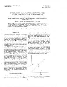
Figure 1. Landmark point-based features are rare in outdoor sporting environments. Instead, one can calibrate the camera using edge-based features by aligning a synthetic view of pitch markings (inset) to a filtered camera image. Our long range gradient permits convergence through gradient-based image alignment, as indicated in the original image.

in urban [6, 15] and rural [16] areas; and sporting facilities [7, 9, 21, 23] (see Figure 1). Lines are more difficult to detect than points, as they require fusing information across multiple pixels. One can estimate the parameters of a line by searching for peaks in Hough space [23], or fitting to a set of image locations (or both [7]). However, each of these methods has inherent difficulties. A Hough transform requires careful selection of quantization scale and nonmaxima suppression [7]; fitting to a set of points requires identifying a subset of pixels from the image to which the line must belong. Curved lines are more problematic, but parametric fits can be computed for some shapes [8]. The image acquisition process introduces additional difficulties. For instance, the large coverage area of outdoor applications means wide-angle lenses will be common. These lenses generally induce distortion into the image making straight lines appear curved [11]. Images captured relatively low to the ground will view features from an oblique angle, which complicates line detection as a double response from an edge filter may be expected or unexpected depending on the width and (unknown) proximity of the line to the camera.

1. Introduction Standard camera calibration algorithms employ a twostage approach which first identifies point correspondences between the image and the world, and then finds parameters which minimize the distance between projected world points and their corresponding image locations [11]. Commonly, a set of feature point correspondences is established by detecting corner-based features within an image of a known calibration object (or adjacent frames if autocalibrating a moving scene). Checkerboards are perhaps the most popular target because of their ease of use and manufacture. In large outdoor scenes, checkerboards are impractical, as the necessary size may be on the order of metres [9, 14]. Furthermore, landmark point features are often rare. Instead, lines and edges are the dominant feature 1

Our method is the first to estimate camera intrinsic, extrinsic and lens distortion parameters by aligning an overhead template to the camera image using gradientbased optimization. Since we do not require a geometric parametrization of the scene (described by detected point, lines and curves in the camera and/or overhead views), we are able to calibrate both the projective and lens parameters simultaneously from arbitrary planar patterns. However, an estimate of the ground to image homography is needed for initialization. Unlike previous image-based calibrations [17,18,22,26], we employ a reduced camera model which assumes known pixel aspect ratio and principal point. This slight restriction vastly improves the robustness of 3D calibration from a 2D surface, as the projective parameters are over determined. Unlike [17], we do not need a 3D model of the scene, nor a complex initialization. We avoid direct image comparisons (and the supplemental parameters needed to account for differences in illumination [18, 26]) by matching the response of an image filter to a geometric template. The camera parameters are estimated by aligning the resulting two edge images (see Figure 1). Finally, we employ a long range gradient which permits aligning two edge images without needing an exhaustive search or iterative multi-scale refinements.

2. Previous Work Image-Based Calibration Image-based calibration estimates camera parameters directly from pixel intensities. A model of the scene including its appearance and geometry (either 2D [12, 26] or 3D [17]) is required. Camera parameters p are estimated by minimizing the difference between a rendered template of the scene and the camera image I. Quite often the process includes auxiliary non-camera parameters to account for additional discrepancies, such as illumination [18, 26]. We avoid additional parameters by aligning to a geometric template image T, which defines the locations of the visual ground plane features. In many outdoor scenarios, such templates are easily available. In sports, an overhead rendering of the pitch is easy to obtain (or produce). In outdoor surveillance, the template could be generated using a filtered satellite image. Kaminsky et al. [15] employed such a strategy for aligning structure from motion point clouds to the world. They conducted a coarse to fine brute force search for the best 2D similarity transform which mapped recovered 3D points to edges in the overhead view. For a given set of camera parameters p, one can generate a greyscale image indicating the portion of each camera pixel xi = (u, v) that overlaps with feature locations. This is equivalent to warping the overhead image T into the camera’s perspective T(W(x; p)), where the warp W(x; p) is determined by projective and lens aspects of the camera (for clarity, we have reversed the convention of [2] and warp the

template, not the image). Assuming one can generate an image I indicating how likely each pixel within the camera’s image corresponds to a visual feature (for instance, a similarity measure based on colour), the optimal set of camera parameters p� can be determined by minimizing the distance between each warped pixel W(xi ; p) and the nearest detected location [13], in much the same fashion that pointbased calibration minimizes projection error. The closest detected pixel in I for a given warped pixel in T may change from one iteration to the next. Gradient-based Image Alignment Although image plane distance is the appropriate error measure to minimize, the difference between T(W(x; p)) and I(x) is nearly equivalent, and is a solvable optimization problem. The forwards additive Lucas-Kanade algorithm [2] finds an optimal set of warp parameters p� through the following iterative steps: 1. Warp T with W(x; p) to compute T (W(x; p)) 2. Compute error image E(x) = I(x) − T (W(x; p)) 3. Warp gradient ∇T with W(x; p) 4. Evaluate Jacobian

∂W ∂p

at (x; p)

5. Compute steepest descent ∇T ∂W ∂p 6. Compute Hessian H = 7. Compute ∆p = H −1 8. Update p ← p + ∆p

� � x

� � x

∇T ∂W ∂p

∇T ∂W ∂p

�T �

�T

∇T ∂W ∂p

�

E(x)

Edge Image Alignment The template image T for outdoor sports scenarios may resemble an edge image. The occurrence of strong edges within an image is relatively rare compared to the number of pixels. This sparseness makes edges difficult to use in gradient-based optimizations [24], as the gradient of an edge filter is effectively non-zero in only a small number of locations (see Figure 2). This means a gradient-based optimizer receives little information about how to modify the current parameters (by ∆p) to reach a better solution. Furthermore, non-zero gradient locations within an edge image may not indicate the quality of the alignment, as one can only judge how well two images align when there is a non-zero difference (the difference between two sparse edge images is zero at most locations). However, the merits of edge features for alignment accuracy and illumination invariance make them worthwhile features for alignment. Cootes and Taylor [5] computed the local orientation of pixels (including a reliability estimate of this measure) to

I(x)

T(W(x; p))

I(x) − T(W(x; p))

∇Tx (W(x; p))

∇Ty (W(x; p))

Figure 2. Edge images are difficult to align, as the image, template and its gradient are all sparse. In this example, the current parameters p warp an edge in T reasonably close to an edge in I (within about 10 pixels). The non-zero elements of the error image indicate how to update ∆p if there is corresponding gradient information in ∇T. However, since the gradient is sparse, there a few pixels which have both non-zero difference and non-zero gradient. As a result, ∆p ≈ 0, and the optimizer is unable to converge to the correct solution.

improve the precision and reliability of fitting models to facial images. Since the process considered the reliability of the orientation estimates, the algorithm focused on aligning strong edge responses between a query image and a model. Optimization was performed in a series of coarse to fine resolutions. Wang et al. [24] also investigated fitting face models to query images. Like Cootes and Taylor, they employed edges (via a Laplacian filter) for better fitting. The optimized parameters were found using an exhaustive local search.

3. Warp Parametrization Lens distorted projective geometry is usually characterized by considering a point x� in the world mapped to a location x in the image plane by a camera projection P(·) (or a homography H(·) for planar geometry) followed by lens distortion L(·). This definition allows one to visualize the camera’s detected features registered to an overhead view, as the reverse mapping is used to compute a warped image [25]. Alignment in this domain would minimize the distance between the locations of the back-projected markings and their expected positions. However, the more common oblique camera angle makes back-projection errors of distant features much more apparent than close ones. As a result, optimized parameters may give good alignment in the overhead domain, but not when projected into the camera image. Minimizing the projection error (instead of the backprojection error) requires the warp to be defined in the opposite direction. Assuming the world co-ordinate x� is described in a planar co-ordinate system, the camera to ground warp W becomes: x� = W(x; p)

= H−1 (L−1 (x; p); p).

(1)

Lens Distortion Model For simplicity, we assume the lens effects are radially symmetric with respect to a distortion centre e, and that the amount of distortion λ at a

particular point within the image depends only on the radial distance. The direction of L — i.e. whether it distorts or undistorts — is arbitrary [20, 22]. For convenience, we define the lens as undistorting and for consistency denote the lens warp as L−1 (x): ˆ = L−1 (x) x

= e + λ(r) (x − e) ,

(2)

ˆ are distorted and undistorted where r = �x−e� and x and x locations in the camera’s image plane. Since λ(r) is an arbitrary function of r ≥ 0, we parametrize it as a Taylor expansion [11], λ(r) = 1 + κ1 r + κ2 r2 + κ3 r3 + · · · + κn rn .

(3)

We fix the centre of distortion e at the centre of the image, which means the lens is parametrized by n lens coefficients, pL−1 = [κ1 , κ2 , . . . , κn ]. (4) The experiments in this paper employ a single lens codef efficient, either κ1 , or κ2 with κ1 = 0 for compatibility with other lens models [3]. It is worth noting that other lens models, such as the rational polynomial expansion [4], could be employed. The only real restriction is that the lens model is parametrizable, unlike [10], and is differentiable. Camera Projection Model Although a perspective camera matrix P = KR[I| − C] has eleven degrees of freedom in general, one can assume some of the intrinsic parameters are known. For instance, a natural camera [11] assumes zero skew and known pixel aspect ratio (typically unity). For simplicity, we assume the principal point coincides with the centre of the image, which means K has only one degree of freedom (the focal length f ), and P has only seven (as there are an additional six to describe 3D position and orientation). If the world co-ordinate system is defined such that z = 0 corresponds to the ground plane, the ground to image

homography H can be extracted from the first, second and fourth columns of the camera projection matrix P (up to a scalar uncertainty). � �T ˆ = P x�x x�y 0 1 x � �� � ∼ xx x�y = KR I | − C

0

1

= Hx� ,

where



1  0 H∼ KR = 0

and

0 1 0

 −Cx −Cy  −Cz

�T

(5)

(6)

(7)

The rotation matrix R describes the camera’s orientation with respect to the world co-ordinate system, and has three degrees of freedom. There are many ways to parametrize R. We chose the Rodrigues axis-angle notation ω = [ωx , ωy , ωz ] which describes R as a rotation of �ω� ˆ Therefore, the projective component radians about axis ω. of W(·) is parametrized by seven elements pH = [f, Cx , Cy , Cz , ωx , ωy , ωz ],

(8)

which is one fewer than the ground to image plane homography of a general projective camera [2].

3.1. Warp Jacobian The image to ground warp W(x; p) is fully characterized by (2), (3) and (7); and directly parametrized by the eight camera parameters. The Jacobian of (1) is computed by applying the chain rule to (7), followed by (2) and (3). To compute the derivative of H−1 , we introduce an intermediate expression G: 

H11 H22 − H12 H21 G =  H12 H20 − H10 H22 H10 H21 − H11 H20

H02 H21 − H01 H22 H00 H22 − H02 H20 H01 H20 − H00 H21

 H01 H12 − H02 H11 H02 H10 − H00 H12  . H00 H11 − H01 H10

−1 The partial derivative of an arbitrary element H−1 ·· of H with respect to parameter pj is then

∂H−1 ·· = ∂pj

∂G·· ∂pj

det H det H − G·· ∂ ∂p j

(det H)2

Intrinsic Matrix For a natural camera with known principal point, the image of the absolute conic (IAC) ω = K−T K−1 has one degree of freedom: the focal length f . The metric ground plane to image plane homography H must satisfy two conditions with respect to the IAC [19]: T T hT 1 ωh1 − h2 ωh2 = 0,

ˆ. x� = H−1 x

def

[11]. Initial values for the seven projective parameters (8) ˆ by estimating the camera’s intrinsic K are extracted from H and extrinsic R[I| − C] matrices. The lens parameters (4) are initialized to zero, which corresponds to ideal pinhole projection.

.

(9)

Details of the remainder of the calculations are provided as supplemental material.

hT 1 ωh2

= 0;

(10) (11)

where hi represents the ith column of H. Therefore, given a metric homography (such as the one estimated via DLT) one can compute K (and therefore f ) from the above system of over determined equations. Extrinsic Matrix The non-perspective components of the homography (6) are recovered by left multiplying H by K−1   1 0 −Cx H� ∼ (12) = K−1 H ∼ = R  0 1 −Cy  . 0 0 −Cz The first two normalized columns of H� will correspond to the first two columns of R. One can estimate the camera’s orientation as � � ˆ� h ˆ� h ˆ� × h ˆ� , (13) R≈ h 1 2 1 2

and then find the closest true orthonormal matrix using SVD [27]. Once R has been estimated, C can be recovered from the third column of H and the Rodrigues vector ω from R. Optimization The ground to image plane homography (6) extracted from the natural camera projection matrix P may be significantly different from the unconstrained homography initially estimated via DLT. As a final initialization step, we optimize the projective warp parameters pH (8) using Levenberg-Marquardt to ensure the homography H extracted from the projection matrix is as close as possiˆ, with both matrices scaled ble to the initial homography H to have unit Frobenius norm.

3.2. Initialization

4. Long Range Gradient

The alignment algorithm is initialized by specifying four point (or line) correspondences between the camera image and the geometric template T. A ground plane to image ˆ is estimated using the DLT algorithm plane homography H and ensuring the cheirality of the estimated matrix is correct

To overcome the narrow convergence range of an edge image (see Figure 2), we compute a gradient of image T at location x by fitting a plane to pixel intensities contained within a (2n + 1) × (2n + 1) window centred at x. The graT dient for location x is given by ∇T(x) = [A, B] , where

0.5

-9

-8

-7

-6

-5

-4

-3

-2

-1

0 dx

1

2

3

4

5

6

7

8

9

10

-10

-9

-8

-7

-6

-5

-4

-3

-2

-1

0 dx

1

2

3

4

5

6

7

8

9

10

-10

-9

-8

-7

-6

-5

-4

-3

-2

-1

0 dx

1

2

3

4

5

6

7

8

9

10

-10

-9

-8

-7

-6

-5

-4

-3

-2

-1

0 dx

1

2

3

4

5

6

7

8

9

10

0.4

Magnitude

-10

0.3

0.2

0.1

0 1 2 3 4 5 6 7 8 9 10 n

Figure 3. (left) A one pixel wide line (black) and its long range gradient evaluated at various locations relative to x for window sizes n = 1, 5 and 9 (indicated using red, green and blue respectively). For illustrative purposes, each gradient response has been normalized relative to its maximum value (right). Note that the response for n = 1 is identical to that of a 3 × 3 Sobel filter. T

the parameters [A B C] of the fitted plane are computed by solving the over-determined system of equations:     −n −n 1 � � T (xx − n, xy − n)  −n + 1

−n .. .

1

A B C

=  T (xx − n +. 1, xy − n) . (14) ..

Fitting parametric models to image intensities is a standard technique for estimating more precise measurements (as discussed in [1]). Here, we deliberately use a large window size to propagate information. In the case of an edge image, approximating the gradient at x by fitting a plane to the nearby intensities is roughly equivalent to a signed distance transform. For example, consider the cross-section of a one pixel wide binary edge response (see Figure 3). For various half-window sizes n, the gradient increases linearly with the distance from x up to its maximum (which occurs at −n). The sign of the gradient indicates the direction towards the centre location x. The gradient at distances sufficiently far from x, i.e. greater than n, is zero. This behaviour preserves the intrinsic robustness of matching edge images (see Figure 2). Suppose the current parameters p warp an edge at x� = W(x; p) in T to location x in I. If x is further than n pixels from the true location x� of the corresponding edge in I, then the non-zero image differences from this misalignment will not contribute to ∆p, as the gradients (and therefore the steepest descents) at x and x� will be zero (see Figure 3). Equivalently, ∆p is only computed from nonzero differences and gradients which are sufficiently close to corresponding edges in I. So, we choose n to be large and refer to this as a long range gradient. For example, Figure 1 was achieved using n = 8, which corresponds to a physical window size of 0.85m.

5. Results The Gauss-Newton image alignment algorithm assumes the warp W(·) is approximately linear for small parameter changes. Lens distorted projection reduces the quality of this assumption. Therefore, we augment the standard forwards additive algorithm with a line search phase: if an estimated parameter update ∆p increases the alignment error, we reduce ∆p by half and re-iterate. As before, the algorithm converges when �∆p� is sufficiently small, or if the maximum number of iterations is exceeded. We compare long range gradients to standard imagebased calibration using field hockey pitch markings, and to traditional feature-based methods using a checkerboard. Field Hockey Images of field hockey pitch markings are difficult to parametrize geometrically. The ‘circle lines’ are constructed from two quarter circles, joined by a straight line segment spanning the width of the goal. The resulting curve is not a conic section. Figure 8 shows a selection of results for a variety of pitches, camera positions and lighting conditions. Our gradient-based method provides significant improvement over the initial ground to image homographies which ignore lens distortion. However, the camera and lens model lacks sufficient complexity to attain pixel perfect alignment. A first order model of pitch curvature may be required for further improvement [23]. The size of the window used for computing long range gradients plays a role in the quality and speed of the optimization process. The overhead view of the pitch markings was rendered at 1 pixel = 0.05m, making one pixel slightly smaller than the width of most pitch markings. The average performance of several of long range gradients were eval-

Relative RMS Image Difference

1 2 4 8 16 32

0.8 0.6 0.4 0.2 0 0

2

4

6

8

10

12

14

16

18

20

22

Iteration

Figure 4. The window size at which long range gradients are computed clearly influences the optimization’s speed and quality. Excessively small or large window sizes lead to sub-optimal alignments. 1.0 0.8 0.6 0.4 0.2 0 0

2

4

6

8

10

12

14

16

18

20

22

Iteration

Figure 5. A long range gradient with n = 4 (solid red) generally converges to a better solution than gradients computed with a 3 × 3 Sobel filter (solid blue). Although a 14 : 12 :1 pyramid (dashed blue) using 3 × 3 Sobel gradients at each level is able to match the performance of a single long range gradient, a sequence n = {4, 2, 1} of contracting long range gradients (dashed red) generally produces the best alignment. 1.0 Average Convergence Rate

Checkerboard We used the MATLAB camera calibration toolbox [3] to generate a reference calibration using twenty images of a 9 × 7 checkerboard. We restricted the intrinsic camera model to estimate only focal length f and a single radial distortion parameter κ2 . For the given test image we computed the camera extrinsic parameters. We compared the proposed image-based alignment to

1.0

Relative RMS Image Difference

uated using seven different field hockey images (see Figure 4). The results illustrate that there is clearly an optimal window size: if n is too small the optimizer is unable to reach parameters far from the initialization; if n is too large, the optimizer cannot make small refinements to p. Image pyramids are often used to minimize the necessity of an optimal window size. Figure 5 illustrates how a pyramid using 3×3 Sobel gradients was generally able to match the precision of a single long range gradient (although after many more iterations). However, like a pyramid, a sequence of contracting long range gradients can similarly reduce the need for an optimal window size (see Figure 6). In our experiments, contracting long range gradients generally produced the best alignment, presumably because contracting long range gradients always use the original data (whereas a pyramid uses down sampled versions). In addition to minimizing the impact of non-optimal window sizes, image pyramids also provide robustness against poor initializations. For each of the seven camera set-ups, we perturbed the image locations of the manually specified correspondences by adding Gaussian random noise. We then optimized using a 18 : 14 : 12 :1 pyramid and a {8, 4, 2, 1} contracting long range gradient sequence. We considered the optimization to have converged if the RMS error was within 10% of the unperturbed solution. Figure 7 illustrates how contracting long range gradients are much more robust to poor initializations.

0.8 0.6 0.4 0.2 0 0

1

2

3

4

5

6

7

8

9

10

Noise Standard Deviation [pixels]

Figure 6. The x-component of successively smaller long range gradients (from bottom to top) computed from the geometric template of field hockey pitch markings.

Figure 7. Gaussian noise was added to each of the four image locations used to initialize the warp parameters. We assumed the optimizer converged to the correct solution if the RMS image difference was within 10% of the unperturbed value. The average rate of convergence over twenty trials for all of the seven camera set-ups demonstrates how an equivalent sequence of contracting long range gradients (red) is quite robust to poor initializations, compared to an equivalent pyramid approach (blue).

Figure 8. Coarse manual initializations (left) were estimated using four point-correspondences. The pitch markings were detected in each image using a colour similarity filter with additional requirements for thin white objects next to green objects. A sequence of contracting long range gradients was used to align the overhead template to the camera’s image (right). Focal Length ∆f [pixels] Reference Calibration

1943

Feature-Based Image-Based

−24 −14

Position �∆C� [m] 

 +0.027  −0.277  −0.291 0.036 0.039

Orientation ˆ ∆ω ∆�ω� [rads] [rads]   0.865161  −0.250564  −0.0355074

−0.0052 −0.0060

0.0030 0.0035

Distortion Error ∆κ2 [ f12 ] [pixels] −0.155

2.45

−0.025 −0.068

4.29 3.93

Table 1. Camera parameters were estimated from the inner 5 × 7 checkerboard (blue dots) using both feature-based and image-based calibration techniques. Both algorithms produce parameter estimates which differ only slightly from the reference calibration (estimated from multiple images). The calibrations were evaluated by comparing the projected positions of the outer checkerboard corners (red dots) to their manually measured locations. Errors significantly larger than the reference calibration are expected, since this is an extrapolation beyond the image region used for calibration.

standard feature-based alignment using a 7 × 5 subset of the 9 × 7 checkerboard (see Table 1). Parameters for the feature-based model were estimated using the same MATLAB calibration toolbox. Each calibration was evaluated by measuring the image plane distance between the projected and detected locations of the remaining 32 corners along the perimeter of the 9 × 7 checkerboard. Since these evaluation points lie outside the domain of points used for calibration, the impact of incorrect parameter estimates will be significant. As expected, both algorithms produce errors approximately 1.5× that of the reference. Both algorithms produce reasonably similar parameters, but image-based calibration has a slightly lower projection error of the test points.

6. Summary Our work formulates camera calibration in terms of image alignment. This is useful when point-based features are not present in the scene. In the majority of images captured outdoors and at sports fields, the dominant visual feature is an edge. Aligning edges images using gradient-based optimization is quite difficult, as the images and gradients are sparse; resulting in a narrow convergence range. We address this issue using a long range gradient. Unlike a pyramid approach, the long range gradient maintains a precise alignment measure, as the image and template are never down sampled. For added robustness, multiple long range gradients may be employed in a pyramid fashion to perform a coarse to fine alignment (when the initialization is far from the solution). For additional robustness, we assume square pixels and known principal point. This is extremely beneficial when calibrating from planes, as the projective parameters are overdetermined. We demonstrate how the image warp W(·) and its Jacobian can be derived from this projection model, including lens distortion. Finally, formulating calibration in terms of image alignment permits the use of arbitrary geometric patterns for calibration.

References [1] S. Baker. Design and Evlauation of Feature Detectors. PhD thesis, Columbia University, 1998. 5 [2] S. Baker and I. Matthews. Lucas-Kanade 20 years on: A unifying framework. IJCV, 56(3):221–255, 2004. 2, 4 [3] J.-Y. Bouguet. Camera calibration toolbox for matlab. 3, 6 [4] D. Claus and A. W. Fitzgibbon. A rational function lens distotion model for general cameras. In CVPR, 2005. 3 [5] T. F. Cootes and C. J. Taylor. On representing edge structure for model matching. In CVPR, pages 1114–1119, 2001. 2 [6] J. Deutscher, M. Isard, and J. MacCormick. Automatic camera calibration from a single manhattan image. In ECCV, 2002. 1 [7] D. Farin, S. Krabbe, P. H. de With, and W. Effelsberg. Robust camera calibration for sport videos using court models. In SPIE Electronic Imaging, pages 80–91, 2004. 1

[8] A. W. Fitzgibbon, M. Pilu, and R. B. Fisher. Direct least square fitting of ellipses. PAMI, 21(5):476–480, 1999. 1 [9] O. Grau, M. Prior-Jones, and G. Thomas. 3d modelling and rendering of studio and sport scenes for tv applications. In WIAMIS, 2005. 1 [10] R. Hartley and S. B. Kang. Parameter-free radial distortion correction with center of distortion estimation. PAMI, 29(8):1309–1321, 2007. 3 [11] R. Hartley and A. Zisserman. Multiple View Geometry in Computer Vision. Cambridge University Press, 2004. 1, 3, 4 [12] H. S. Hong and M. J. Chung. 3D pose and camera parameter tracking algorithm based on Lucas-Kanade image alignment algorithm. In International Conference on Control, Automatic and Systems, 2007. 2 [13] D. P. Huttenlocher, G. A. Klanderman, and W. J. Rucklidge. Comparing images uisng the hausdorff distance. PAMI, 15(9):850–863, 1993. 2 [14] Y. Kameda, T. Takemasa, and Y. Ohta. Outdoor mixed reality utilizing surveillance cameras. In SIGGRAPH, 2004. 1 [15] R. S. Kamensky, N. Snavely, S. M. Seitz, and R. Szeliski. Alignment of 3D point clouds to overhead images. In Second IEEE Workshop on Internet Vision, 2009. 1, 2 [16] B. Majidi and A. Bab-Hadiashar. Aerial tracking of elongated objects in rural environments. Machine Vision and Applications, 20:23–34, 2009. 1 [17] L. Robert. Camera calibration without feature extraction. CVIU, 63(2):314–325, 1996. 2 [18] H. S. Sawhney and R. Kumar. True multi-image alignment and its application to mosaicing and lens distortion correction. PAMI, 21(3):235–243, 1999. 2 [19] P. Sturm and S. Maybank. On plane-based camera calibration: A general algorithm, singularities, applications. In CVPR, volume 1, page 437 Vol. 1, 1999. 4 [20] R. Szeliski. Image alignment and stitching: a tutorial. Foundations and Trends in Computer Graphics and Vision, 2(1):1–104, 2006. 3 [21] F. Szenberg, P. Carvalho, and M. Gattass. Automatic camera calibration for image sequences of a football match. In Advances in Pattern Recognition, pages 303–312, 2001. 1 [22] T. Tamaki, T. Yamamura, and N. Ohnishi. Unified approach to image distortion. In ICPR, 2002. 2, 3 [23] G. Thomas. Real-time camera tracking using sports pitch markings. Real-Time Image Processing, 2:117–132, 2007. 1, 5 [24] Y. Wang, S. Lucey, and J. Cohn. Non-rigid object alignment with a mismatch template based on exhaustive local search. In IEEE Workshop on Non-rigid Registration and Tracking through Learning, October 2007. 2, 3 [25] G. Wolberg. Digital Image Warping. IEEE Computer Society Press, 1992. 3 [26] G. Ye, M. Pickering, M. Frater, and J. Arnold. Efficient multi-image registration with illumination and lens distortion correction. In ICIP, 2005. 2 [27] Z. Zhang. A flexible new technique for camera calibration. PAMI, 22(11):1330–1334, 2000. 4