CAMLS: A Constraint-based Apriori Algorithm for Mining Long Sequences Yaron Gonen1 ,
[email protected], Nurit Gal-Oz1 ,
[email protected], Ran Yahalom1 ,
[email protected], and Ehud Gudes1 ,
[email protected] Computer Science, Ben Gurion University of the Negev, Israel
Abstract. Mining sequential patterns is a key objective in the field of data mining due to its wide range of applications. Given a database of sequences, the challenge is to identify patterns which appear frequently in different sequences. Well known algorithms have proved to be efficient, however these algorithms do not perform well when mining databases that have long frequent sequences. We present CAMLS, Constraint-based Apriori Mining of Long Sequences, an efficient algorithm for mining long sequential patterns under constraints. CAMLS is based on the apriori property and consists of two phases, event-wise and sequence-wise, which employ an iterative process of candidate-generation followed by frequency-testing. The separation into these two phases allows us to: (i) introduce a novel candidate pruning strategy that increases the efficiency of the mining process and (ii) easily incorporate considerations of intra-event and inter-event constraints. Experiments on both synthetic and real datasets show that CAMLS outperforms previous algorithms when mining long sequences.
1
Introduction
The sequential pattern mining task has received much attention in the data mining field due to its broad spectrum of applications. Examples of such applications include analysis of web access, customers shopping patterns, stock markets trends, DNA chains and so on. This task was first introduced by Agrawal and Srikant in [1]: Given a set of sequences, where each sequence consists of a list of elements and each element consists of a set of items, and given a user-specified min support threshold, sequential pattern mining is to find all of the frequent subsequences, i.e. the subsequences whose occurrence frequency in the set of sequences is no less than min support. In recent years, many studies have contributed to the efficiency of sequential mining algorithms [12, 8, 1, 4, 3]. The two major approaches for sequence mining arising from these studies are: apriori and sequence growth. The apriori approach is based on the apriori property, as introduced in the context of association rules mining in [7]. This property states that if a pattern α is not frequent then any pattern β that contains α cannot be frequent. Two of the most successful algorithms that take this approach are GSP [8] and SPADE [12].
The major difference between the two is that GSP uses a horizontal data format while SPADE uses a vertical one. The sequence growth approach does not require candidate generation, it gradually grows the frequent sequences. PrefixSpan [4], which originated from FP-growth [2], uses this approach as follows: first it finds the frequent single items, then it generates a set of projected databases, one database for each frequent item. Each of these databases is then mined recursively while concatenating the frequent single items into a frequent sequence. These algorithms perform well in databases consisting of short frequent sequences. However, when mining databases consisting of long frequent sequences, e.g. stocks values, DNA chains or machine monitoring data, their overall performance exacerbates by an order of magnitude. Incorporating constraints in the process of mining sequential patterns, is a means to increase the efficiency of this process and to obviate ineffective and surplus output. cSPADE [11] is an extension of SPADE which efficiently considers a versatile set of syntactic constraints. These constraints are fully integrated inside the mining process, with no post-processing step. Pei et al. [5] also discuss the problem of pushing various constraints deep into sequential pattern mining. They identify the prefix-monotone property as the common property of constraints for sequential pattern mining and present a framework (Prefix-growth) that incorporates these constraints into the mining process. Prefix-growth leans on the sequence growth approach [4]. In this paper we introduce CAMLS, a constraint-based algorithm for mining long sequences, that adopts the apriori approach. The motivation for CAMLS emerged from the problem of aging equipment in the semiconductor industry. Statistics show that most semiconductor equipment suffer from significant unscheduled downtime in addition to downtime due to scheduled maintenance. This downtime amounts to a major loss of revenue. A key objective in this context is to extract patterns from monitored equipment data in order to predict its failure and reduce unnecessary downtime. Specifically, we investigated lamp behavior in terms of illumination intensity that was frequently sampled over a long period of time. This data yield a limited amount of possible items and potentially long sequences. Consequently, attempts to apply traditional algorithms, resulted in inadequate execution time. CAMLS is designed for high performance on a class of domains characterized by long sequences in which each event is composed of a large number of items. CAMLS consists of two phases, event-wise and sequence-wise, which employ an iterative process of candidate-generation followed by frequency-testing. The event-wise phase discovers frequent events satisfying constraints within an event (e.g. two items that cannot reside within the same event). The sequence-wise phase constructs the frequent sequences and enforces constraints between events within these sequences (e.g. two events must occur one after another within a specified time interval). This separation allows the introduction of a novel pruning strategy which reduces the size of the search space considerably. We aim to utilize specific constraints that are relevant to the class of domains for
which CAMLS is designed. Experimental results compare CAMLS to known algorithms and show that its advantage increases as the mined sequences get longer and the number of frequent patterns in them rises. The major contributions of our algorithm are its novel pruning strategy and straightforward incorporation of constraints. This is what essentially gives CAMLS its high performance, despite of the large amount of frequent patterns that are very common in the domains for which it was designed. The rest of the paper is organized as follows. Section 2 describes the class of domains for which CAMLS is designed and section 3 provides some necessary definitions. In section 4 we characterize the types of constraints handled by CAMLS and in section 5 we formally present CAMLS. Experimental results are presented in section 6. We conclude by discussing future research directions.
2
Characterization of Domain Class
The classic domain used to demonstrate sequential pattern mining, e.g. [1], is of a retail organization having a large database of customer transactions, where each transaction consists of customer-id, transaction time and the items bought in the transaction. In domains of this class there is no limitation on the total number of items, or the number of items in each transaction. Consider a different domain such as the stock values domain, where every record consists of a stock id, a date and the value of the stock on closing the business that day. We know that a stock can have only a single value at the end of each day. In addition, since a stock value is numeric and needs to be discretized, the number of different values of a stock is limited by the number of the discretization bins. We also know that a sequence of stock values can have thousands of records, spreading over several years. We classify domains by this sort of properties. We may take advantage of prior knowledge we have on a class of domains, to make our algorithm more efficient. CAMLS aims at the class of domains characterized as follows: – Large amount of frequent patterns due to: • Very long sequences. • A potentially large number of items in each event. – There is a relatively small number of frequent events. Table 1 shows an example sequence database that will accompany us throughout this paper. It has three sequences. The first contains three events: (acd), (bcd) and b in times 0, 5 and 10 respectively. The second contains three events: a, c and (db) in times 0, 4 and 8 respectively, and the third contains three events: (de), e and (acd) in times 0, 7 and 11 respectively. In section 6 we present another example concerning the behavior of a QuartzTungsten-Halogen lamp, which has similar characteristics and is used for experimental evaluation. Such lamps are used in the semiconductors industry for finding defects in a chip manufacturing process.
Table 1: Example sequence database. Every entry in the table is an event. The first column is the identifier of the sequence that the event belongs to. The second column is the time difference from the beginning of the sequence to the occurrence of the event. The third column shows all of the items that constitute the event. Sequence id Event id (sid) (eid) 1 0 1 5 1 10 2 0 2 4 2 8
3
items (acd) (bcd) b a c (bd)
Sequence id Event id items (sid) (eid) 3 0 (cde) 3 7 e 3 11 (acd)
Definitions
An item is a value assigned to an attribute in our domain. We denote an item as a letter of the alphabet: a, b, ..., z. Let I = {i1 , i2 , ..., im } be the set of all possible items in our domain. An event is a nonempty set of items that occurred at the same time. We denote an event as (i1 , i2 , ..., in ), where ij ∈ I, 1 ≤ j ≤ n. An event containing l items is called an l-event. For example, (bcd) is a 3-event. If every item of event e1 is also an item of event e2 then e1 is said to be a subevent of e2 , denoted e1 ⊆ e2 . Equivalently, we can say that e2 is a superevent of e1 or e2 contains e1 . For simplicity, we denote 1-events without the parentheses. Without the loss of generality we assume that items in an event are ordered lexicographically, and that there is a radix order between different events. Notice that if an event e1 is a proper superset of event e2 then e2 is radix ordered before e1 . For example, the event (bc) is radix ordered before the event (abc), and (bc) ⊆ (abc). A sequence is an ordered list of events, where the order of the events in the sequence is the order of their occurrences. We denote a sequence s as he1 , e2 , ..., ek i where ej is an event, and ej−1 happened before ej . Notice that an item can occur only once in an event but can occur multiple times in different events in the same sequence. A sequence containing k events is called a k-sequence, in contrast to the classic definition of k-sequence that refers to any sequence containing k items® [8]. For example, h(de)e(acd)i is a 3-sequence. A® sequence s1 = e11 , e12 , ..., e1n is a subsequence of sequence s2 = e21 , e22 , ..., e2m , denoted s1 ⊆ s2 , if there exists a series of integers 1 ≤ j1 < j2 < ... < jn ≤ m such that e11 ⊆ e2j1 ∧e12 ⊆ e2j2 ∧...∧e1n ⊆ e2jn . Equivalently we say that s2 is a super-sequence of s1 or s2 contains s1 . For example habi and h(bc)f i are subsequence of ha(bc)f i, however h(ab)f i is not. Notice that the subsequence relation is transitive, meaning that if s1 ⊆ s2 and s2 ⊆ s3 then s1 ⊆ s3 . An m-prefix of an n-sequence s is any subsequence of s that contains the first m events of s where m ≤ n. For example, ha(bc)i is a 2-prefix of ha(bc)a(cf )i. An m-suffix of an n-sequence s is any subsequence of s that contains the last m events of s where m ≤ n. For example, h(cf )i is a 1-suffix of ha(bc)a(cf )i.
A database of sequences is an unordered set of sequences, where every sequence in the database has a unique identifier called sid. Each event in every sequence is associated with a timestamp which states the time duration that passed from the beginning of the sequence. This means that the first event in every sequence has a timestamp of 0. Since a timestamp is unique for each event in a sequence it is used as an event identifier and called eid. The support or frequency of a sequence s, denoted as sup(s), in a sequence database D is the number of sequences in D that contain s. Given an input integer threshold, called minimum support, or minSup, we say that s is frequent if sup(s) ≥ minSup. The frequent patterns mining task is to find all frequent subsequences in a sequence database for a given minimum support.
4
Constraints
A frequent patterns search may result in a huge number of patterns, most of which are of little interest or useless. Understanding the extent to which a pattern is considered interesting may help in both discarding ”bad” patterns and reducing the search space which means faster execution time. Constraints are a means of defining the type of sequences one is looking for. In their classical definition [1], frequent sequences are defined only by the number of times they appear in the dataset (i.e. frequency). When incorporating constraints, a sequence must also satisfy the constraints for it to be deemed frequent. As suggested in [5], this contributes to the sequence mining process in several aspects. We focus on the following two: (i) Performance. Frequent patterns search is a hard task, mainly due to the fact that the search space is k extremely large. For example, with d items there are O(2d ) potentially frequent sequences of length k. Limiting the searched sequences via constraints may dramatically reduce the search space and therefore improve the performance. (ii) Non-contributing patterns. Usually, when one wishes to mine a sequence database, she is not interested in all frequent patterns, but only in those meeting certain criteria. For example, in a database that contains consecutive values of stocks, one might be interested only in patterns of very profitable stocks. In this case, patterns of unprofitable stocks are considered non-contributing patterns even if they are frequent. By applying constraints, we can disregard noncontributing patterns. We define two types of constraints: intra-event constraints, which refer to constraints that are not time related (such as values of attributes) and inter-events constraints, which relate to the temporal aspect of the data, i.e. values that can or cannot appear one after the other sequentially. For the purpose of the experiment conducted in this study and in accordance with our domain, we chose to incorporate two inter-event and two intra-events constraints. A formal definition follows. Intra-event Constraints – Singletons Let A = {A1 , A2 , ...An } s.t. Ai ⊆ I, be the set of sets of items that cannot reside in the same event. Each Ai is called a singleton. For example,
the value of a stock is an item, however a stock cannot have more than one value at the same time, therefore, the set of all possible values for that stock is a singleton. – MaxEventLength The maximum number of items in a single event. Inter-events Constraints – MaxGap The maximum amount of time allowed between consecutive events. A sequence containing two events that have a time gap which is grater than MaxGap, is considered uninteresting. – MaxSequenceLength The maximum number of events in a sequence.
5
The Algorithm
We now present CAMLS, a Constraint-based Apriori algorithm for Mining Long Sequences, which is a combination of modified versions of the well known Apriori [1] and SPADE [12] algorithms. The algorithm has two phases, event-wise and sequences-wise, which are detailed in subsections 5.1 and 5.2, respectively. The distinction between the two phases corresponds to the difference between the two types of constraints. As explained below, this design enhances the efficiency of the algorithm and makes it readily extensible for accommodating different constraints. Pseudo code for CAMLS is presented in Algorithm 1.
Algorithm 1 CAMLS Input minSup: minimum support for a frequent pattern. maxGap: maximum time gap between consecutive events. maxEventLength: maximum number of items in every event. maxSeqLength: maximum number of events in a sequence. D: data set. A: set of singletons. Output F : the set of all frequent sequences. procedure CAMLS(minSup, maxGap, maxEventLength , maxSeqLength, D, A) 1: {Event-wise phase} 2: F1 ← allFrequentEvents(minSup, maxEventLength, A, D) 3: F ← F1 4: {Sequence-wise phase} 5: for all k such that 2 ≤ k ≤ maxSeqLength and Fk−1 6= φ do 6: Ck ←candidateGen(Fk−1 , maxGap) 7: Fk ←prune(Fk−1 , Ck , minSup, maxGap) 8: F ← F ∪ Fk 9: end for 10: return F
5.1
Event-wise Phase
The input to this phase is the database itself and all of the intra-event constraints. During this phase, the algorithm disregards the sequential nature of the data, and treats the data as a set of events rather than a set of sequences. Since the data is not sequential, applying the intra-event constraints at this phase is very straightforward. The algorithm is similar to the Apriori algorithm for discovering frequent itemsets as presented in [1]. Similarly to Apriori, our algorithm utilizes an iterative approach where frequent (k − 1)-events are used to discover frequent k-events. However, unlike Apriori, we calculate the support of an event by counting the number of sequences that it appears in rather than counting the number of super-events that contain it. This means that the appearance of an event in a sequence increases its support by one, regardless of the number of times that it appears in that sequence. Denoting the set of frequent k-events by Lk (referred to as frequent k-itemsets in [1]), we begin this phase with a complete database scan in order to find L1 . Next, L1 is used to find L2 , L2 is used to find L3 and so on, until the resulting set is empty, or we have reached the maximum number of items in an event as defined by MaxEventLength. Another difference between Apriori and this phase lies in the generation process of Lk from Lk−1 . When we join two (k−1)-events to generate a k-event candidate we need to check whether the added item satisfies the rest of the intra-event constraints such as Singletons. The output of this phase is a radix ordered set of all frequent events satisfying the intra-event constraints, where every event ei is associated with an occurrence index. The occurrence index of the frequent event ei is a compact representation of all occurrences of ei in the database and is structured as follows: a list li of sids of all sequences in the dataset that contain ei , where every sid is associated with the list of eids of events in this sequence that contain ei . For example, Figure 1a shows the indices of events d and (cd) based on the example database of Table 1. We are able to keep this output in main memory due to the nature of our domain in which the number of frequent events is relatively small. Since the support of ei equals the number of elements in li , it is actually stored in ei ’s occurrence index. Thus, support is obtained by querying the index instead of scanning the database. In fact, the database scan required to find L1 is actually the only single scan of the database. Throughout the event-wise phase, additional scans are avoided by keeping the occurrence indices for each event. The allF requentEvents procedure in line 2 of Algorithm 1 is responsible for executing the event-wise phase as described above. 5.2
Sequence-wise Phase
The input to this phase is the output of the previous one. It is entirely temporalbased, therefore applying the inter-events constraints is straightforward. The output of this phase is a list of frequent sequences satisfying the inter-events
(a) The occurrence indices of events d and (cd) from the example database of Table 1. Event d occurs in sequence 1 at timestamps 0 and 5, in sequence 2 at timestamp 8 and in sequence 3 at timestamps 0 and 11. Event (cd) occurs in sequence 1 at timestamps 0 and 5 and in sequence 3 at timestamps 0 and 11.
(b) Example of the occurrence index for sequence < d(cd) > generated from the intersection of the indices of sequences < d > and < (cd) >.
Fig. 1: Example of occurrence index.
constraints. Since it builds on frequent events that satisfied the intra-event constraints, this output amounts to the final list of sequences that satisfy the complete set of constraints. Similarly to SPADE [12], this phase of the algorithm finds all frequent sequences by employing an iterative candidate generation method based on the apriori property. For the k th iteration, the algorithm outputs the set of frequent k-sequences, denoted as Fk , as follows: it starts by generating the set of all ksequence candidates, denoted as Ck from Fk−1 (found in the previous iteration). Then it prunes candidates that do not require support calculation in order to determine that they are non-frequent. Finally, it calculates the remaining candidates’ support and removes the non-frequent ones. The following subsections elaborate on each of the above steps. This phase of the algorithm is a modification of SPADE in which the candidate generation process is accelerated. Unlike SPADE, that does not have an event-wise phase and needs to generate the candidates at an item level (one item at a time), our algorithm generates the candidates at an event level, (one event at a time). This approach can be significantly faster because it allows us to use an efficient pruning method(section 5.2) that would otherwise not be possible. Candidate Generation We now describe the generation of Ck from Fk−1 . For each pair of sequences s1 , s2 ∈ Fk−1 that have a common (k − 2)-prefix, we conditionally add two new k-sequence candidates to Ck as follows: (i) if s1 is a generator (see section 5.2), we generate a new k-sequence candidate by concatenating the 1-suffix of s2 to s1 ; (ii) if s2 is a generator, we generate a new k-sequence candidate by concatenating the 1-suffix of s1 to s2 . It can be easily proven that if Fk−1 is radix ordered then the generated Ck is also radix ordered. For example, consider the following two 3-sequences: h(ab)c(bd)i and h(ab)cf i. Assume that these are frequent generator sequences from which we want to generate 4-sequence candidates. The common 2-prefix of both 3sequences is h(ab)ci and their 1-suffixes are h(bd)i and hf i. The two 2-sequences
Algorithm 2 Candidate Generation Input Fk−1 : the set of frequent (k − 1)-sequences. Output Ck : the set of k-sequence candidates. procedure candidateGen(Fk−1 ) 1: for all sequence s1 ∈ Fk−1 do 2: for all sequence s2 ∈ Fk−1 s.t. s2 6= s1 do 3: if pref ix(s1 ) = pref ix(s2 ) then 4: if isGenerator(s1 ) then 5: c ← concat(s1 , suf f ix(s2 )) 6: Ck ← Ck ∪ {c} 7: end if 8: if isGenerator(s2 ) then 9: c ← concat(s2 , suf f ix(s1 )) 10: Ck ← Ck ∪ {c} 11: end if 12: end if 13: end for 14: end for 15: return Ck
we get from the concatenation of the 1-suffixes are h(bd)f i and hf (bd)i. Therefore, the resulting 4-sequence candidates are h(ab)cf (bd)i and h(ab)c(bd)f i. Pseudo code for the candidate generation step is presented in Algorithm 2. Candidate Pruning Candidate generation is followed by a pruning step. Pruned candidates are sequences identified as non-frequent based solely on the apriori property without calculating their support. Traditionally, [12, 8], k-sequence candidates are only pruned if they have at least one (k − 1)-subsequence that is not in Fk−1 . However, our unique pruning strategy enables us to prune some of the k-sequence candidates for which this does not apply, due to the following observation: in the k th iteration of the candidate generation step, it is possible that one k-sequence candidate will turn out to be a super-sequence of another k-sequence. This happens when events of the subsequence are contained in the corresponding events if we have of the super-sequence. ® More formally, ® the two k-sequences s1 = e11 , e12 , ..., e1k and s2 = e21 , e22 , ..., e2k then s1 ⊆ s2 if e11 ⊆ e21 ∧ e12 ⊆ e22 ∧ ... ∧ e1k ⊆ e2k . If s1 was found to be non-frequent, s2 can be pruned, thereby avoiding the calculation of its support. For example, if the candidate haaci is not frequent, we can prune h(ab)aci, which was generated in the same iteration. Our pruning algorithm is decribed as follows. We iterate over all candidates c ∈ Ck in an ascending radix order (this does not require a radix sort of Ck because its members are generated in this order - see section 5.2). For each c, we check whether all of its (k − 1)-subsequences are in Fk−1 . If not, then c is not frequent and we add it to the set Pk which is a radix ordered list of pruned k-sequences that we maintain throughout the pruning step. Otherwise, we check
whether a subsequence cp of c exists in Pk . If so then again c is not frequent and we prune it. However, in this case, there is no need to add c to Pk because any candidate that would be pruned by c will also be pruned by cp . Note that this check can be done efficiently since it only requires O(log(|Pk |) · k) comparisons of the events in the corresponding positions of cp and c. Furthermore, if there are any k-subsequences of c in Ck that need to be pruned, the radix order of the process ensures that they have been already placed in Pk prior to the iteration in which c is checked. Finally, if c has not been pruned, we calculate its support. If c has passed the minSup threshold then it is frequent and we add it to Fk . Otherwise, it is not frequent, and we add it to Pk . Pseudocode for the candidate pruning is presented in Algorithm 3. Support Calculation In order to efficiently calculate the support of the ksequence candidates we generate an occurrence index data structure for each candidate. This index is identical to the occurrence index of events, except that the list of eids represent candidates and not single events. A candidate is represented by the eid of the last event in it. The index for candidate s3 ∈ Ck is generated by intersecting the indices of s1 , s2 ∈ Fk−1 from which s3 is derived. Denoting the indices of s1 , s2 and s3 as inx1 , inx2 and inx3 respectively, the index intersection operation inx1 ⊙ inx2 = inx3 is defined as follows: for each pair sid1 ∈ inx1 and sid2 ∈ inx2 , we denote their associated eids list as eidList(sid1 ) and eidList(sid2 ), respectivly. For each eid1 ∈ eidList(sid1 ) and eid2 ∈ eidList(sid2 ), where sid1 = sid2 and eid1 < eid2 , we add eid2 to eidList(sid1 ) as new entry in inx3 . For example, consider the 1-sequences s1 =< d > and s2 =< (cd) > from the example database of Table 1. Their indices, inx1 and inx2 , are described in Figure 1a. The index inx3 for the 2sequence s3 =< d(cd) > is generated as follows: (i) for sid1 =1 and sid2 =1, we have eid1 =0 and eid2 =5 which will cause sid=1 to be added to inx3 and eid=5 to be added to eidList(1) in inx3 ; (ii) for sid1 =3 and sid2 =3, we have eid1 =0 and eid2 =11 which will cause sid=3 to be added to inx3 and eid=11 to be added to eidList(3) in inx3 . The resulting inx3 is shown in Figure 1b. Notice that the support of s3 can be obtained by counting the number of elements in the sid list of inx3 . Thus, the use of the occurrence index enables us to avoid any database scans which would otherwise be required for support calculation. Handling the MaxGap Constraint Consider the example database in Table 1, with minSup = 0.5 and maxGap = 5. Now, let us look at the following three 2-sequences: habi, haci, hcbi, all in C2 and have a support of 2 (see section 5.3 for more details). If we apply the maxGap constraint, the sequence habi is no longer frequent and will not be added to F2 . This will prevent the algorithm from generating hacbi, which is a frequent 3-sequence that does satisfy the maxGap constraint. To overcome this problem, during the support calculation, we mark frequent sequences that satisfy the maxGap constraint as generators. Sequences that do not satisfy the maxGap constraint, but whose support is higher than minSup, are marked as non-generators and we refrain from pruning
them. In the following iteration we generate new candidates only from frequent sequences that were marked as generators. The procedure isGenerator in Algorithm 3 returns the mark of a sequence (i.e., whether it is a generator or not). Algorithm 3 Candidate Pruning Input Fk−1 : the set of frequent (k − 1)-sequences. Ck : the set of k-sequence candidates. minSup: minimum support for a frequent pattern. maxGap: maximum time gap between consecutive events. Output Fk : the set of frequent k-sequence. procedure prune(Fk−1 , Ck , minSup, maxGap) 1: Pk ← φ 2: for all candidates c ∈ Ck do 3: isGenerator(c) ← true; 4: if ∃s ⊆ c ∧ s is a (k − 1)-sequence ∧s ∈ / Fk−1 then 5: Pk .add(c) 6: continue 7: end if 8: if ∃cp ∈ Pk ∧ cp ⊂ c then 9: continue 10: end if 11: if !(sup(c) ≥ minSup) then 12: Pk .add(c) 13: else 14: Fk .add(c) 15: if !(c satisfies maxGap) then 16: isGenerator(c) ← false; 17: end if 18: end if 19: end for 20: return Fk
5.3
Example
Consider the sequence database D given in Table 1 with minSup set to 0.6 (i.e. 2 sequences), maxGap set to 5 and the set {a, b} is a Singleton. Event-wise phase. Find all frequent events in D. They are: h(a)i : 3, h(b)i : 2 , h(c)i : 3 , h(d)i : 3 , h(ac)i : 2, h(ad)i : 2, h(bd)i : 2, h(cd)i : 2 and h(acd)i : 2, where h(event)i : support represents the frequent event and its support. Each of the frequent events is marked as a generator, and together they form the set F1 . Sequence-wise phase. This phase iterates over the the candidates list until no more candidates are generated. Iteration 1, step 1: Candidate generation. F1 performs a self join, and 81 candidates are generated: haai, habi , haci, ..., ha(acd)i, hbai, hbbi, ..., h(acd)(acd)i. Together they form C2 . Iteration 1, step 2: Candidate pruning. Let us consider the candidate haai. All its 1-subsequences appear in F1 , so the Fk−1 pruning passes. Next, P2 still does not contain any
sequences, so the Pk pruning passes as well. However, it does not pass the frequency test, since its support is 0, so haai is added to P2 . Now let us consider the candidate ha(ac)i. It passes the Fk−1 pruning, however, it does not pass the Pk pruning since a subsequence of it, haai, appears in P2 . Finally, let us consider the candidate hbci. It passes both Fk−1 and Pk pruning steps. Since it has a frequency of 2 it passes the frequency test, however, it does not satisfy the maxGap constraint, so it is marked as a non-generator, but added to F2 . All the sequences marked as generators in F2 are: haci : 2, hcbi : 2, hcdi : 2 and hc(bd)i : 2. The other sequences in F2 are marked as non-generators and are: habi : 2, hadi : 2, ha(bd)i : 2, hdci : 2, hddi : 2 and hd(cd)i : 2. Iteration 2 At the end of this iteration, only one candidate passes all the pruning steps: hacbi : 2, and since no candidates can be generated from one sequences, the process stops.
6
Experimental Results
In order to evaluate the performance of CAMLS, we implemented SPADE, PrefixSpan (and its constrained version, Prefix-growth) and CAMLS in Java 1.6 using the Weka [10] platform. We compared the run-time of the algorithms by applying them on both synthetic and real data sets. We conducted several runs with and without including constraints. Since SPADE does not incorporate constraints we have excluded it from the latter runs. All tests were conducted on an AMD Athlon 64 processor box with 1GB of RAM and a SATA HD running Windows XP. The synthetic datasets mimic real-world behavior of a Quartz-
SYN10−5
SYN30−3 CAMLS SPADE PrefixSpan
1.5
80
120
140
2.0
100
SYN10−3
4643
80
40
60
31
Runtime(seconds)
170 80 27
Runtime(seconds)
460
1.0
Runtime(seconds)
60
100
10855
0.5
40
7431
20
20
1961
3835
621
2599
33
171
0.8
0.7
0.6
Minimum Suppor t
0.5
0
0
0.0
368 0.9
0.9
0.8
0.7
0.6
Minimum Suppor t
0.5
0.9
0.8
0.7
0.6
0.5
Minimum Suppor t
Fig. 2: Execution-time comparisons between CAMLS, SPADE and PrefixSpan on synthetic datasets for different values of minimum support, without constraints.
Tungsten-Halogen lamp. Such lamps are used in the semiconductors industry for finding defects in a chip manufacturing process. Each dataset is organized in a table of synthetically generated illumination intensity values emitted by a lamp. A row in the table represents a specific day and a column represents a specific wave-length. The table is divided into blocks of rows where each block represents a lamp’s life cycle, from the day it is first used to the last day it worked
R30
R100
21957
307199
0.3
0.2
1e+02 Runtime(seconds)
82 14 2
582 2
1e−02
1e+00
0.05 0.10 0.20
0.50 1.00 2.00
CAMLS SPADE PrefixSpan
0.01 0.02
Runtime(seconds)
5.00
2531
0.5
0.4
0.3
Minimum Support
0.2
0.5
0.4
Minimum Support
Fig. 3: Execution-time comparisons between CAMLS, SPADE and PrefixSpan on two real datasets for different values of minimum support, without constraints.
right before it burned out. To translate this data into events and sequences, the datasets were preprocessed as follows: first, the illumination intensity values were discretized into 50 bins using equal-width discretization [6]. Next, 5 items were generated: (i) the highest illumination intensity value out of all wave-lengths, (ii) the wave-length at which the highest illumination intensity value was received (iii) an indication whether or not the lamp burned out at the end of that day, (iv) the magnitude of the light intensity gradient between two consecutive measurements and (v) the direction of the light intensity gradient between two consecutive measurements. We then created two separate datasets. For each row in the original dataset, an event consisting of the first 3 items was formed for the first dataset and an event consisting of all 5 items was formed for the second one. Finally, in each dataset, a sequence was generated for every block of rows representing a lamp’s life cycle from the events that correspond to these rows. We experimented with four such datasets each containing 1000 sequences and labeled SYNα-β where α stands for the sequence length and β stands for the event length. The real datasets, R30 and R100, were obtained from a repository of stock values [9]. The data consists of the values of 10 different stocks at the end of the business day, for a period of 30 or 100 days, respectively. The value of a stock for a given day corresponds to an event and the data for a given stock corresponds to a sequence, thus giving 10 sequences of either 30 (in R30) or 100 (in R100) events of length 1. As a preprocessing step, all numeric stock values were discretized into 50 bins using equal-frequency discretization [6]. Figure 2 compares CAMLS, SPADE and PrefixSpan on three synthetic datasets without using constraints. Each graph shows the change in execution-time as the minimum support descends from 0.9 to 0.5. The amount of frequent patterns found for each minimum support value is indicated by the number that appears above the respective bar. This comparison indicates that CAMLS has a slight advantage on datasets of short sequences with short events(SYN10-3). However, on datasets containing longer events (SYN10-5) and long sequences (SYN30), the advantage of CAMLS becomes more pronounced as the amount of frequent patterns rises when decreasing the minimum support (around 5% faster than PrefixSpan and 35% faster than SPADE on the avarage). Similar results can
SYN30−5
R100
40
100
SYN30−3
CAMLS
140
Prefix−growth
51351
80
Runtime(seconds)
4643
Runtime(seconds)
20
Runtime(seconds)
60
100
30
80
120
3901
10
40
40
60
2021
1961
1209
20
21957
621 171
20
33
519
129
0.8
0.7
0.6
Minimum Suppor t
0.5
582
0
0
0
1 0.9
0.9
0.8
0.7
0.6
Minimum Suppor t
0.5
0.5
0.4
0.3
0.2
Minimum Suppor t
Fig. 4: Execution-time comparisons between CAMLS and Prefix-growth on SYN30-3 SYN30-5 and R100 with the maxGap and Singletons constraints for different values of minimum support.
be seen in Figure 3 which compares CAMLS, SPADE and PrefixSpan on the two real datasets. In R30, SPADE and PrefixSpan has a slight advantage over CAMLS when using high minimum support values. We believe that this can be attributed to the event-wise phase that slows CAMLS down, compared to the other algorithms, when there are few frequent patterns. On the other hand, as the minimum support decreases, and the number of frequent patterns increases, the performance of CAMLS becomes better in an order of magnitude. In the R100 dataset, where sequences are especially long, CAMLS clearly outperforms both algorithms for all minimum support values tested. In the extreme case of the lowest value of minimum support, the execution of SPADE did not even end in a reasonable amount of time. Figure 4 compares CAMLS and Prefix-growth on SYN30-3, SYM30-5 and R100 with the usage of the maxGap and Singletons constraints. On all three datasets, CAMLS outperforms Prefix-growth.
7
Discussion
In this paper we have presented CAMLS, a constraint-based algorithm for mining long sequences, that adopts the apriori approach. Many real-world domains require a substantial lowering of the minimum support in order to find any frequent patterns. This usually amounts to a large number of frequent patterns. Furthermore, some of these datasets may consist of many long sequences. Our motivation to develop CAMLS originated from realizing that well performing algorithms such as SPADE and PrefixSpan could not be applied on this class of domains. CAMLS consists of two phases reflecting a conceptual distinction between the treatment of temporal and non temporal data. Temporal aspects are only relevant during the sequence-wise phase while non temporal aspects are dealt with only in the event-wise phase. There are two primary advantages to this distinction. First, it allows us to apply a novel pruning strategy which accelerates the mining process. The accumulative effect of this strategy becomes especially apparent in the presence of many long frequent sequences. Second, the incorporation of inter-event and intra-event constraints, each in its associated phase,
is straightforward and the algorithm can be easily extended to include other inter-events and intra-events constraints. We have shown that the advantage of CAMLS over state of the art algorithms such as SPADE, PrefixSpan and Prefixgrowth, increases as the mined sequences get longer and the number of frequent patterns in them rises. We are currently extending our results to include different domains and compare CAMLS to other algorithms. In future work, we plan to improve the CAMLS algorithm to produce only closed sequences and to make our pruning strategy even more efficient.
References 1. Rakesh Agrawal and Ramakrishnan Srikant. Mining sequential patterns. In ICDE ’95: Proceedings of the Eleventh International Conference on Data Engineering, pages 3–14, Washington, DC, USA, 1995. IEEE Computer Society. 2. Jiawei Han, Jian Pei, Yiwen Yin, and Runying Mao. Mining frequent patterns without candidate generation: A frequent-pattern tree approach. Data Min. Knowl. Discov., 8(1):53–87, 2004. 3. Heikki Mannila, Hannu Toivonen, and A. Inkeri Verkamo. Discovery of frequent episodes in event sequences. Data Min. Knowl. Discov., 1(3):259–289, 1997. 4. Jian Pei, Jiawei Han, Senior Member, Behzad Mortazavi-asl, Jianyong Wang, Helen Pinto, Qiming Chen, Umeshwar Dayal, Ieee Computer Society, Ieee Computer Society, and Mei chun Hsu. Mining sequential patterns by pattern-growth: The prefixspan approach. IEEE Transactions on Knowledge and Data Engineering, 16:2004, 2004. 5. Jian Pei, Jiawei Han, and Wei Wang. Constraint-based sequential pattern mining: the pattern-growth methods. J. Intell. Inf. Syst., 28(2):133–160, 2007. 6. Dorian Pyle. Data preparation for data mining. Morgan Kaufmann Publishers Inc., San Francisco, CA, USA, 1999. 7. Ramakrishnan Srikant Rakesh Agrawal. Fast algorithms for mining association rules. In Jorge B. Bocca, Matthias Jarke, and Carlo Zaniolo, editors, Proc. 20th Int. Conf. Very Large Data Bases, VLDB, pages 487–499. Morgan Kaufmann, 12–15 1994. 8. R. Srikant and R. Agrawal. Mining sequential patterns: Generalizations and performance improvements. In Advances in Database Technology–EDBT’96: 5th International Conference on Extending Database Technology, Avignon, France, March 25-29, 1996: Proceedings, page 3. Springer, 1996. 9. Luis Torgo. Daily stock prices from january 1988 through october 1991, for ten aerospace companies., 2007. 10. Ian H. Witten and Eibe Frank. Data mining: practical machine learning tools and techniques with java implementations. SIGMOD Rec., 31(1):76–77, 2002. 11. Mohammed J. Zaki. Sequence mining in categorical domains: incorporating constraints. In CIKM ’00: Proceedings of the ninth international conference on Information and knowledge management, pages 422–429, New York, NY, USA, 2000. ACM. 12. Mohammed J. Zaki. Spade: An efficient algorithm for mining frequent sequences. In Machine Learning, pages 31–60, 2001.