The use of the neural networks to estimate software development effort has been viewed with skepticism by the majority of the cost estimation community.
Can Neural Networks be easily Interpreted in Software Cost Estimation?
Ali Idri, Taghi M. Khoshgoftaar, Alain Abran
Abstract The use of the neural networks to estimate software development effort has been viewed with skepticism by the majority of the cost estimation community. Although, neural networks have shown their strengths in solving complex problems, their shortcoming of being ‘black boxes’ has prevented them to be accepted as a common practice for cost estimation. In this paper, we study the interpretation of cost estimation models based on a Back-propagation three multilayer Perceptron network. Our idea consists in the use of a method that maps this neural network to a fuzzy rule-based system. Consequently, if the obtained fuzzy rules are easily interpreted, the neural network will also be easy to interpret. Our experiment is made using the COCOMO’81 dataset.
1. Introduction Estimation models in software engineering are used to predict some important attributes of future entities such as software development effort, software reliability, and productivity of programmers. Among these models, those estimating software effort have motivated considerable research in recent years. The prediction procedure used by these software-effort models can be based on a mathematical function, such as Effort = α × size β or other techniques such as artificial neural networks, analogy based reasoning, regression trees, and rule induction models. In this paper, we are concerned with cost estimation models that are based on artificial neural networks. The artificial neural networks approach is inspired from biological nerve nets. An artificial neural network is characterized by its architecture, its learning algorithmic and its activation functions. In general, for software cost estimation, the most commonly adopted architecture, learning algorithm and activation function are respectively the feed-forward multi-layer Perceptron, the Back-propagation algorithm and the Sigmoid function. Many researchers have applied the neural networks approach to estimate software development effort [5,13,16,17,18,19,20,21].Most of their investigations have
focused more attention on the accuracy of the approach when compared to other cost estimation techniques. Table 1 shows a summary of artificial neural networks effort prediction studies. There are two main advantages when using estimation by artificial neural networks. First, it allows the learning from previous situations and outcomes. The learning criteria is very important for cost estimation models because software development technology is supposed to be continuously evolving. Second, it can model a complex set of relationships between the dependent variable (such as, cost or effort) and the independent variables (cost drivers). However, there are some shortcomings that prevent it from being accepted as a common practice in cost estimation (Are there some specific references that have identified these shortcomings, or is this something new?): § Neural networks approach may be considered as ‘black boxes’. Consequently, it is not easy to understand and to explain its process to the users. § The ability of neural networks to solve problems of high complexity has been proven in classification and categorization areas whereas in the cost estimation field we deal with a generalization rather than a classification problem. § There is no guidelines for the construction of the neural networks topologies (number of layers, number of units per layer, initial weights, …) In this work, we deal with the first limitation. Many researchers in different fields refuse to use neural nets because of their shortcoming of being ‘black boxes’, that is determining why an artificial neural networks makes a particular decision is a difficult task. This is a significant weakness, for without the ability to produce comprehensive (understandable – explainable, comprehensible or something related??) decisions, it is hard to trust the reliability of networks addressing real-world problems. Consequently, we are convinced that the explanation and the interpretation of the knowledge stored in the architecture and the synapse weights of the neural nets is very important to gain practitioners acceptance. Our idea consists in the use of a method that maps one neural
2002 World Congress on Computational Intelligence, Honolulu, Hawaii, May 12-17, 2002
1
network to an equivalent Fuzzy Rule-Based System (FRBS). Consequently, if the obtained if-then fuzzy rules are easily interpreted, then the neural network may also be easily interpreted. Our experiment will be based on the COCOMO’81 historical dataset. This paper is organized as follows: In Section 2, we present how the neural networks approach has been applied to software cost estimation. We present also the architecture of the network that will be used in our experiment. In Section 3, we discuss the results obtained when using the network to estimate the software development effort. In Section 4, we briefly outline the principle of the Benitez’s method that will be used to extract the if-then fuzzy rules from our network. In Section 5, we apply the Benitez’s method to our network and we discuss the interpretation of the obtained fuzzy rules in software cost estimation. A conclusion and an overview of future work conclude this paper.
2. Artificial neural networks for software cost estimation Many different models of neural networks have been proposed [13]. They may be grouped in two major categories. First, feed-forward networks where no loops in the network path occur. Second, feedback networks that have recursive loops. The feed-forward multi-layer perceptron with Back-propagation learning algorithm are the most commonly used in the cost estimation field. In these nets, neurons are arranged in layers and there are only connections between neurons in one layer to the following. Figure 1 illustrates possible network architecture configured for software development effort estimation. The network generates output (effort) by propagating the initial inputs (cost drivers or project attributes) through subsequent layers of processing elements to the final output layer. Each neuron in the network computes a nonlinear function of its inputs and passes the resultant value along its output. The favored function is the Sigmoid function:
Study Venkatachalam Wittig &Finnie Jorgenson Serluca Samson et al. Sarnivasan & Fisher Hughes
Learning algorithm Back-propagation Back-propagation
Dataset
f ( x) =
1 1 + e−x
(1)
Before the network will be ready to make estimates for new projects, it is trained by a set of combination of inputs and outputs that are known as the training data. Our experiment consists in estimating the software development effort by using the neural networks approach on the COCOMO’81 dataset. The COCOMO’81 dataset contains 63 software projects [2,3,4]. Each project is described by 17 attributes: the software size measured in KDSI (Kilo Delivered Sources Instructions), the project mode is defined as either ‘organic’, ‘semi-detached’ or ‘embedded’, and the remaining 15 attributes are measured on a scale composed of six linguistic values: ‘very low’, ‘low’, ‘nominal’, ‘high’, ‘very high’, and ‘extra-high’. Among these 17 attributes, we have retained the KDSI and 12 other attributes that we had already fuzzified [6]. The other attributes are not used in our experiment because their description proved insufficient for fuzzification. The fuzzy sets associated to each selected attribute will be used in the interpretation of the if-then fuzzy rules deduced from our neural network. Input layer
Hidden layer
Output layer
wij KDSI
βj
RELY
Effort
ACAP AEXP
SCED
Figure 1: A neural network architecture for software development effort
Number Of projects 63 81 136 109 28 63 78
Predicting
COCOMO Development effort Desharnais/ Effort ASMA Back-propagation Jorgenson Maintenance effort Back-propagation Mermaid-2 Development effort Back-propagation COCOMO Development effort Back-propagation Kemerer & Development effort COCOMO Back-propagation Hughes 33 Development effort Table 1: Summary of neural network studies [17]
2002 World Congress on Computational Intelligence, Honolulu, Hawaii, May 12-17, 2002
Results Promising MMRE=17% MMRE=100% MMRE=76% MMRE=428% MMRE=70% MMRE=55%
2
The use of the neural network approach to estimate the software effort requires certain decisions and choices about the architecture, learning algorithm and the activation functions. In our case, the method, that we use to generate the if-then fuzzy rules from the neural network, requires that the architecture must be three multi-layer perceptron with the activation functions of the hidden layer and the output layer are respectively the sigmoid and the identity functions. Our neural network has 13 inputs (COCOMO cost drivers) and one output (effort). All the inputs as well as the output of the network are numeric (but it was said in a previous section that they were linguistic and then fuzzified. – there is an apparent contradiction, or a logical link not clear enough). All inputs are normalized to speed up the training process of the network [14]. The network is trained by iterating through the training data many times. The used algorithm is Back-propagation with teaching rate and maximum error are equals to 0,03 and 10-5, respectively. Finally, Back-propagation assumes that weights in the network are initialized to small, random values prior to training. According to the architecture of our network, the effort (output) is given by: h
Effort = ∑ z j β j j =1
n
with
z j = f (∑ wij xi ) i =1
where f is the sigmoid function, wij are the weights of the connections from the inputs layer to the hidden layer and βj are those from the hidden layer to the output layer.
3. Overview of the empirical results The following section presents and discusses the results obtained when applying our neural network to the COCOMO’81 dataset. The calculations were made using a software prototype developed with the C language under a PC Microsoft Windows. The accuracy of the estimates is evaluated by using the magnitude of relative error MRE defined as: MRE =
Effortactual − Effortestimated Effortactual
The MRE is calculated for each project in the dataset. In addition, we use the measure prediction level Pred. This measure is often used in the literature. It is defined by: k Pr ed ( p ) = N where N is the total number of historical projects, k is the number of new projects with an MRE less than or equal to p. A common value for p is 0.25. The Pred(0.25) gives the percentage of projects that were predicted with an MRE equal or less than 0.25. Other four quantities are used in
this evaluation: min of MRE, max of MRE, median of MRE, and mean of MRE (MMRE). We have conducted several experiments to choose (randomly ???) the number of hidden units (it is not clear to the unspecialised reader, what is a 'unit' and the related concepts, and its importance – this is very important to understand since this is mentioned often in the subsequent sections of the text). These experiments use the full COCOMO’81 dataset for training and testing the network. An acceptable accuracy is obtained with 13 hidden units and 300,000 learning iterations (Table 2). MRE%
NN with 13 hidden units and 300,000 learning iterations Max 16,67 Mean 1,50 Min 0,00 Table 2: Estimates accuracy of a network with 13 hidden units
However, many studies have proved that the neural network approach generates less accurate estimates when the training data is different from the test data [18,19]. Three reasons explain this phenomenon: § The new project is widely different from the projects that are used in the training phase § The number of projects used in the training phase is insufficient § There is no relationship between the chosen cost drivers (inputs of the network) and the effort (output of the network) To back this affirmation, we have conducted two different experiments with our neural network. In the first experiment, we have randomly removed 23 projects from the COCOMO’81 dataset. These 23 projects are used to test the network. The 40 remaining projects are used to train the network. In the second experiment, we have removed only one project that is used for testing and we use all the remaining projects for training. The removed project is one of the 23 removed projects in the first experiment. The second experiment is repeated 23 times. Table 3 shows the obtained results for the two experiments. The values of MRE and pred(25) prove that, in general, the accuracy is increasing with the number of projects used in the training phase.
Pred(25) MMRE % Med MRE % Min MRE %
NN with 40 projects for training 13,04 203,66 92,53 2,6
2002 World Congress on Computational Intelligence, Honolulu, Hawaii, May 12-17, 2002
NN with 62 projects for training 34,78 84,35 53,67 2,84
3
Max MRE % 1188,89 432,5 Table 3: Estimates accuracy of a network with 40 and 62 projects in the training phase. As we have noticed, in this work, we are not concerned with the accuracy of our network. The aim is to explain its process by mapping the network to a fuzzy rule-based system. The method developed by Benitez et al. will be used to extract the if-then fuzzy rules from our network [1]. In the next section, we present this method.
fuzzy set with the membership function is the sigmoid function of the hidden units. The number of the fuzzy rules Rjk is equal to the number of hidden units. In order to make the fuzzy rules Rjk easily interpreted, Benitez et al. have shown that each of them can be given by:
R jk : if x1 is A1jk ∗ x 2 is A 2jk ∗ ... ∗ x n is A njk then y k = β jk where A ijk are fuzzy sets obtained from A and wij. Their membership functions are given by:
µ Ai ( x ) = µ A ( xw ij ) jk
4. Equivalence between neural networks and fuzzy rules-based systems: Background Since its foundation by Zadeh in 1965 [22], fuzzy logic has been the subject of many investigations. One of its main contributions to solve complex problems is undoubtedly the Fuzzy Rule-Based Systems. Basically, an FRBS is based on a set of if-then fuzzy rules1. A fuzzy rule is an if-then statement where the premise and the consequence consist of fuzzy propositions whereas in a classical production rule the premise and the consequence are crisp. An example of fuzzy rule in cost estimation may be ‘if the competence of the analysts is high then the effort is low’. The main advantage of fuzzy rules over classical rules is that they are more understandable for humans and may be easily interpreted. Indeed, fuzzy rules use, unlike classical rules, in their premises and consequences linguistic values instead of numerical data. As a consequence, some researches have investigated the equivalence between neural networks and FBRS’s [1,11 (11 is not the correct reference here)]. These investigations have the objective to translate the knowledge embedded in the neural network into a more understandable language that is the if-then fuzzy rules. Benitez et al. have developed a method that proves the equality between a neural network, such as the one used in the previous section, and a fuzzy rule-based system which uses Sugeno rules [1]. In the following section, we present this method. Let us consider a three-layer perceptron neural network with the sigmoid function for the hidden units and the identity function for the output unit. This three-layer perceptron neural network is equal to a fuzzy rule-based system that uses a set of fuzzy rules Rjk associated to all pairs of its units (hidden, output). n
R jk : if ∑ xi wij is A then y k = β jk i =1
where xi are the inputs, yk is the output, wij are the weights of the inputs units to the hidden units, βjk are the weights of the hidden units to the output unit and A is a 1
Details of the FBRS are beyond the scope of this paper. In addition to the rule base, an FBRS is composed of other three parts: fuzzifier, inference engine and defuzzifier.
and * is the i-or operator defined by:
i − or ( a1 , a 2 ,..., a n ) =
a1 a 2 ...a n (1 − a1 )(1 − a 2 )...(1 − a n ) + a1 a 2 ...a n
The i-or operator is an hybrid between T-norm and Tconorm. The fuzzy proposition x is A ijk may be interpreted as ‘x is approximately greater than 2,2/wij’ if wij is positive or ‘x is approximately not greater than 2,2/-wij’ if wij is negative.
5. Validation and interpretation of the fuzzy rules In this section, we apply the method developed by Benitez et al. on the neural network presented and discussed in Sections 2 and 3. The neural network that we consider has 13 hidden units and uses the full COCOMO’81 dataset for training. Consequently, the rule base obtained is composed of 13 fuzzy rules. Each fuzzy rule contains 13 fuzzy propositions. Each one is associated to one cost driver (inputs of the network). The output of each fuzzy rule is a numerical value (positive or negative). These 13 fuzzy rules express the knowledge encoded into the synaptic w eights of our network. The objective is to give a more comprehensible interpretation of these fuzzy rules in software cost estimation by using our previous experiments [6,7,8,9,10,11]. For simplicity, we discuss only two fuzzy rules (Table 4). By analyzing these two rules, we notice that the output of the first rule, R1, is positive (6049,77) whereas the one of the second rule, R2, is negative (-2979,21). These two values are among the synapse weights of the hidden layer to the output units. Consequently, the natural interpretation that we can give of the output of the 13 fuzzy rules is that they can be considered as partial contributions to the total effort. They have the same role as the effort multipliers in the COCOMO’81 model. They can increase (positive value) or decrease (negative value) the total effort. The only difference between them is that the outputs of the fuzzy rules are positive or negative, because the cost function of the FBRS uses the summation operator, whereas in the COCOMO’81 model the effort multipliers
2002 World Congress on Computational Intelligence, Honolulu, Hawaii, May 12-17, 2002
4
are higher than 1 (increase the effort) or lower than 1(decrease the effort) because the COCOMO’81 cost function uses the multiplication operator.
R1:
R2:
If : DATA VIRTmi TIME STORE VIRTma TURN ACAP AEXP PCAP VEXP LEXP SCED KDSI Then
If : is approximately greater than is approximately not greater than is approximately not greater than is approximately not greater than is approximately not greater than is approximately not greater than is approximately not greater than is approximately not greater than is approximately not greater than is approximately not greater than is approximately not greater than is approximately not greater than is approximately not greater than Y=6049,77
117,57 30,14 156,28 155,72 448,88 25,76 203,72 400,37 331,69 1958,86 921,91 794,68 132,27
DATA VIRTmi TIME STORE VIRTma TURN ACAP AEXP PCAP VEXP LEXP SCED KDSI Then
is approximately greater than is approximately not greater than is approximately greater than is approximately not greater than is approximately greater than is approximately not greater than is approximately not greater than is approximately not greater than is approximately not greater than is approximately greater than is approximately greater than is approximately not greater than is approximately greater than Y=-2979,21
118,46 18,14 3716,39 573,41 1232,53 46,33 393,35 272,94 483,23 1357,35 985,36 171,20 176,79
Table 4 : Two examples of the obtained fuzzy rules
0,9
0,5
0,5 0,1 117,57
30,14
(a)
(b)
Figure 2: (a) Fuzzy set associated to the qualification ‘approximately greater than 117,57’. (b) Fuzzy set associated to the qualification ‘approximately not greater than 30,14’ The premise of each fuzzy rule is composed of 13 fuzzy propositions combined by the i-or operator. Each proposition is expressed by a statement such as ‘x is approximately greater than v’ or ‘x is approximately not greater than v’. The linguistic qualification ‘approximately greater than v’ is represented by a fuzzy set with membership function of the equation 1. The value v is the one for which the membership function has a degree equal to 0,9 in case of ‘approximately greater’ or to 0,1 in case of ‘approximately not greater’. According to Benitez et al., the values 0,1 and 0,9 are used in neural literature to indicate respectively the total absence of activation and full activation of the neurons. In our case, all the numerical values of the 13 inputs of the network are positive. Thus, we use only the positive part of the domain of the fuzzy sets corresponding to the qualification ‘approximately (not) greater than’. Figure 2 shows two examples that illustrate
the fuzzy sets used in the two first propositions of the rule R1. The interpretation of each fuzzy proposition depends on the meaning of the cost driver used by this proposition. For instance, the fuzzy proposition ‘DATA is approximately
D Database size in bytes or characters = P Pr ogram size in DSI greater than 117,57’ uses the DATA cost driver which is measured in the COCOMO’81 model by the following ratio (Figure 3): The DATA attribute represents, with other three cost drivers, the effect of the size and the complexity of the database on the software development effort. Thus, the higher the value of DATA, the more it will increase the
2002 World Congress on Computational Intelligence, Honolulu, Hawaii, May 12-17, 2002
5
total effort. By using our fuzzification of the DATA attribute, we notice that the value 117,57 belongs to the linguistic value ‘high’ [6]. Consequently, the fuzzy proposition ‘DATA is approximately greater than 117,57’ may be considered as equivalent to the proposition ‘DATA is high or very high’. The latest proposition is easily understood by cost estimation community. However, in many fuzzy rules obtained, the value, v, used in the proposition ‘x is approximately (not) greater than v’ is out of the range values allowed for one cost driver. For example, in the first fuzzy rule R1, the proposition ‘LEXP is approximately not greater than 921,91’ uses a value (921,91), which is not in the interval of all possible values of the LEXP attribute. Indeed, LEXP represents the programming language experience of the programmers and it is measured by the number of months of experience. In the COCOMO’81 model, the higher allowed value is equal to 36 months. By using our fuzzification of the LEXP attribute, the proposition ‘LEXP is approximately not greater than 921,91’ of the rule R1 may be considered as equivalent to ‘LEXP is Q(very low)’ where Q is a linguistic modifier such as ‘more’. In this example, we have ignored the parts of the area of the fuzzy set representing ‘approximately not greater than 921,91’ which overlap with the linguistic values ‘low’, ‘nominal’ and ‘high’ (Figure 4). The same situation discussed above can be presented for the linguistic qualification ‘approximately greater than’. For example, the proposition ‘LEXP is approximately greater than 985,36’ of the rule R2 may be considered as equivalent to the proposition ‘LEXP is Q(high)’ where Q is a linguistic modifier such as ‘very’ or ‘extra’. Up to now, we have suggested a natural interpretation of the premises and the outputs of the obtained fuzzy rules. It Low
still remains to explain the meaning of the i-or operator that is used to combine the fuzzy propositions of the premises. According to Benitez et al., the i-or operator has a natural interpretation and may be used in the evaluation of many real-world situations (evaluation of scientific papers, evaluation of the quality of a game developed by two tennis players,…). By analyzing all the 13 obtained fuzzy rules, it seems that the i-or operator is not appropriate to evaluate the effect of the premises on the effort. Indeed, the effect of one premise on the effort is calculated by considering all those associated to the 13 cost drivers. In cost estimation, the effect of one cost driver on the effort depends on its type (monotonous increasing or decreasing) and its importance. Moreover, according to its definition and its properties, the i-or operator cannot adequately model the complex set of relationships existing between the cost drivers. There are other reasons that prevent the i-or operator to be easily interpreted: § It is neither a t-norm nor a t-conorm operator. Also, there is no linguistic quantifier that can express its meaning § Let us consider that the truth value of one fuzzy proposition is closer to 1 and for all others their truth values are in the vicinity of 0. In such situation, when combining the various truth values by the i-or operator, the firing (???) strength of the rule will be closer to 1. This is in contradiction with our intuition, especially if the fuzzy proposition that have the truth value closer to 1 contains the less important cost driver. § The i-or operator has the value 0.5 as a neutral element whereas if the truth value of one fuzzy proposition is equal to 0.5, the proposition must contribute in the evaluation of the firing strength of the premise.
Nominal
High
Very High
1
5
55
10
550 100 1000 Figure 3: Membership functions of fuzzy sets defined for the DATA cost driver [6]
Very Low
Low
Nominal
D/P
High
Approximately not greater than 921,91 0,5
0,5
1
2
4
8
12
36
2002 World Congress on Computational Intelligence, Honolulu, Hawaii, May 12-17, 2002
921,91
6
Figure 4: Example where the value used for the LEXP attribute is out of range values
6. Conclusion and future work In this paper, we have studied one of the most important limitations of neural networks, that is understanding why an neural network makes a particular decision is a difficult task. Our study is intended for the cost estimation field. The neural network that we have used to predict the software development effort is the Back-propagation three multi-layer perceptron with sigmoid function in the hidden units and the identity function in the output unit. We have used the full COCOMO’81 dataset to train and to test the network. The obtained accuracy of the network is acceptable. After training and testing the network, we have applied the Benitez’s method to extract the if-then fuzzy rules from this network. These fuzzy rules express the information encoded in the architecture of the network. The interpretation of each fuzzy rule is made by analyzing its premise and its output. Our experiment shows that we can explain the meaning of the output and the propositions composing the premise of each fuzzy rule. However, the i-or operator seems to be inappropriate to combine the effects of the various fuzzy propositions on the output of the fuzzy rule (rule's' ???) in software cost estimation. Consequently, we are looking now to the use of other methods in order to extract more comprehensible (understandable ??) fuzzy rules from the type of neural network used in this experiment (????). 7. Bibliography [1] J. M. Benitez, J.L. Castro, I. Requena, ’Are Artificial Neural Networks Black Boxes?’, IEEE Transaction on Neural Networks, Vol. 8, NO. 5, September, 1997, pp. 1156-1164 [2] B.W. Boehm, Software Engineering Economics, PrenticeHall, 1981. [3] B.W. Boehm, and al., “Cost Models for Future Software Life Cycle Processes: COCOMO 2.0”, Annals of Software Engineering on Software Process and Product Measurement, Amsterdam, 1995. [4] D.S. Chulani, “Incorporating Bayesian Analysis to Improve the Accuracy of COCOMO II and Its Quality Model Extension”, Ph.D. Qualifying Exam Report, USC, February, 1998. [5] R.T Hughes, ‘An Evaluation of Machine Learning Techniques for Software Effort Estimation’, University of Brighton, 1996 [6] A. Idri, L. Kjiri, and A. Abran, “COCOMO Cost Model Using Fuzzy Logic”, 7th Intenational Conference on Fuzzy Theory & Technology, Atlantic City, NJ, February, 2000. pp. 219-223
[7] A. Idri, and A. Abran, “Towards A Fuzzy Logic Based Measures For Software Project Similarity”, Sixth Maghrebian Conference on Computer Sciences, Fes, Morroco, November, 2000. pp. 9-18 [8] A. Idri, and A. Abran, “A Fuzzy Logic Based Measures For Software Project Similarity: Validation and Possible Improvements”, 7th International Symposium on Software Metrics, IEEE computer society,4-6 April, England, 2001. pp. 85-96 [9] A. Idri, and A. Abran, “Evaluating Software Project Similarity by using Linguistic Quantifier Guided Aggregations”, 9th IFSA World Congress/20th NAFIPS International Conference, 25-28 July, Vancouver, 2001. pp. 416-421 [10] A. Idri, A. Abran, T. M. Khoshgoftaar, “Fuzzy Analogy: A new Approach for Software Cost Estimation”, 11th International Workshop in Software Measurements, 28-29 August, Montreal, 2001, pp. 93-101 [11] A. Idri, T. M. Khoshgoftaar, A. Abran, , “Estimating Software Project Effort by Analogy based on Linguistic values”, To be presented in 8th IEEE International Software Metrics Symposium”, 4-7 Ottawa, Canada, 2002 [12] J. S. Jang, C. T. Sun, ‘Functional equivalence between radial basis function networks and fuzzy inference systems’, IEEE Transaction on Neural Networks, Vol. 4, 1992, pp. 156158 [13] M Jorgersen, ‘Experience with Accuracy of Software Maintence Task Effort Prediction Models’, IEEE Transaction on Software Engineering, Vol. 21(8), 1995, pp. 674-681 [14] A. Lapedes, Farber R., ‘Nonlinear signal prediction using neural networks’, Prediction and System modeling’, Los Alamos National Laboratory, Tech. Report, LA-UR-87-2662, 1987 [15] R. P. Lippman, , ‘An Introduction to computing with neural nets’, IEEE ASSP Mag, vol. 4, pp.4-22, 1987 [16] B. Samson, Ellison D., Dugard P, ‘Software Cost Estimation using an Albus Perceptron’, 8th International COCOMO Estimation meeting, Pittsburgh, 1993 [17] C. Schofield, ‘Non-Algorithmic Effort Estimation Techniques’, Tech. Report TR98-01, March, 1998 [18] C. Serluca, ‘An Investigation into Software Effort Estimation using a Back-propagation Neural Network, M.Sc. Thesis, Bournemouth University, 1995 [19] K. Srinivasan, Fisher D, ‘Machine Learning Approaches to Estimating Softawre Development Effort’, IEEE Transaction on Software Engineering, Vol. 21, No. 2, February, 1995, pp. 126-136 [20] A. R. Verkatachalam, ‘Software Cost Estimation using Artificial Neural Networks, International Joint Conference on Neural Networks, Nogoya, IEEE, 1993 [21] G. Wittig, G. Finnie, ‘Estimating Software Development Effort with connectionist Models’, Information and Software Technologie, vol. 39, 1997, pp. 469-476 [22] L.A. Zadeh, “Fuzzy Set”, Information and Control, Vol. 8, 1965, pp. 338-353
2002 World Congress on Computational Intelligence, Honolulu, Hawaii, May 12-17, 2002
7
8