cember 2007. 15. Rüdiger Dillmann, Oliver Rogalla, Markus Ehrenmann, Raoul D Zöllner, and Monica Bor- ... Gillian Hayes and John Demiris. A robot controller ...
Can We Learn Finite State Machine Robot Controllers from Interactive Demonstration? Daniel H Grollman and Odest Chadwicke Jenkins
Abstract There is currently a gap between the types of robot control polices that can be learnt from interactive demonstration and those manually programmed by skilled coders. Using regression-based robot tutelage, robots can be taught previously unknown tasks whose underlying mappings between perceived world states and actions are many-to-one. However, in a finite state machine controller, multiple subtasks may be applicable for a given perception, leading to perceptual aliasing. The underlying mapping may then be one-to-many. To learn such policies, users are typically required to provide additional information, such as a decomposition of the overall task into subtasks, and possibly indications of where transitions occur. We examine the limits of a regression-based approach for learning an FSM controller from demonstration of a basic robot soccer goal-scoring task. While the individual subtasks can be learnt, full FSM learning from this data will require techniques for model selection and data segmentation. We discuss one possibility for addressing these issues and how it may be combined with existing work.
1 Introduction We investigate regression-based interactive Robot Learning from Demonstration (RLfD) for use in instantiating a soccer-style goal-scoring Finite State Machine (FSM) controller on a robot dog and conclude that overlaps between subtasks make the underlying regression problem ill-posed. In order to fully learn the FSM controller, additional information such as the segmentation of data into subtasks must be given. Without this information, we are limited to learning many-to-one (unimap) policies, resulting in a divide between policies that can be taught, and those that can be programmed, as visualized in Figure 1. It may, however, be possible to derive the Daniel H Grollman · Odest Chadwicke Jenkins Brown University, 115 Waterman Street, Providence RI 02912-1910 e-mail: {dang,cjenkins}@cs.brown.edu
1
2
Daniel H Grollman and Odest Chadwicke Jenkins
Fig. 1: An illustration of the gap between robot control policies that are currently learnable from interactive, regression based learning from demonstration, and those manually programmed by skilled coders. Particularly, finite state machine controllers may result in perceptual aliasing and cause learned behaviors to differ from those desired. Hand coded controllers can deal with this aliasing and perform correctly.
needed subtask information from the demonstration data itself, by performing both model selection (choosing the number of subtasks) and data segmentation (the allocation of data to subtasks) at the same time. Policies for these discovered subtasks and transitions between them may then be learnt with existing methods, providing for full FSM learning from collected perception-actuation tuples. More broadly, our aim is to perform Human-Robot Policy Transfer (HRPT), the realization of decision-making control policies for robots representative of a human user’s intended robot behavior. As robots and the tasks they perform become more complicated, it is possible that traditional programming techniques will be overwhelmed. Learning from Demonstration (LfD, sometimes called Programming by Demonstration or Learning by Imitation) is a technique that may enable nonprogrammers to imbue robots with new capabilities throughout its lifetime [28]. Formally, LfD for HRPT is the estimation of a policy π(ˆs) → a, a mapping from perceived states to actions, from demonstrations of a desired task. Data (D = {ˆsi , ai }) is limited to pairs of experienced perception and demonstrated actions, from which ˆ In the absence of a demonstrator, this learning forms an approximated policy, π. learned policy can be used to control the robot. Within RLfD, there are multiple possible approaches for actually inferring πˆ from D. One method is to assume a known parametric model for the task’s control policy. Learning is then the estimation of parameters for this model from the human demonstration. Approximations in the model may be dealt with by learning additional higher-level task-specific parameters [3]. An alternative technique is to use demonstrated trajectories as constraints on an underlying reward signal that the user is assumed to be attempting to maximize, in a form of Inverse Reinforcement Learning. Several techniques can then be used to find a policy that maximizes this discovered reward function [32]. By modeling the
Can We Learn Finite State Machine Robot Controllers from Interactive Demonstration?
3
reward function directly, this approach can enable robots to perform better than their demonstrators, as in acrobatic helicopter flight [1]. In interactive learning for discrete action spaces, Confidence-Based Autonomy [9] uses classification to segment the robot’s perception space into areas where different actions are applicable. This is a form of Direct Policy Approximation, where the policy itself is learned without intermediate steps [43]. This specific approach has been extended to consider situations where the correct action is ambiguous, but the possibilities are equivalent [8]. Here we will use the same interactive robot learning technique, or tutelage, where the user trains the robot, immediately observes the results of learning, and can incrementally provide new demonstrations to improve task performance [22]. This paradigm differs from that of batch training, where all data is gathered before learning occurs, which itself takes place offline over extended periods of time. A major advantage of tutelage is its ability to generate targeted data. That is, the demonstrator only needs to provide demonstrations of the portions of the task that the learner fails to execute properly, which become evident as the robot behaves. The user does not, therefore, need to anticipate what portions of the task will be difficult to learn. Our use of learning, to approximate the control policy, is in contrast to those which learn a model (dynamic or kinematic) of the robot itself, which can then be used for decision making [33]. We pursue learning for decision making as one difficulty of HRPT is that the true robot policy desired by the user is latent in their mind and may be difficult to express through traditional computer programming. It may further be challenging to formulate an appropriate reward function or control basis for the task itself. LfD offers a compelling alternative for HRPT, allowing users to implicitly instantiate policies through examples of task performance [15, 21]. This chapter is organized as such: This section introduced the robot tutelage paradigm, and Section 2 discusses learning tasks composed of multiple subtasks. Section 3 presents the architecture we use, Dogged Learning, and explains how learning takes place. In Section 4 we present one regression-based learning approach and show experiments in using it to learn our scoring task in Section 5. We examine the issue of perceptual aliasing in Section 6 and present a workaround for use with standard regression, along with our thoughts on a possible new approach to simultaneous model selection, data segmentation, and subtask learning. We conclude in Section 7 with an answer to our titular question.
2 Subtasks We consider tasks formed from multiple subtasks, such as a finite state machine, where each machine state is an individual subtask. Learning a full FSM from demonstration can be divided into three aspects: 1. Learn the number of FSM states (subtasks). 2. Learn their individual policies. 3. Learn the transitions between them.
4
Daniel H Grollman and Odest Chadwicke Jenkins
(a) Full FSM learning
(b) Transition learning
(c) Policy learning
Fig. 2: a) The three steps in learning an FSM. Learn the subtasks (boxes), their policies (letters), and the transitions between them (lines). Dashed lines and question marks indicate unknown quantities. Previous work has learned transitions given policies (b), or policies given transitions (c).
An optional additional step is to improve the performance of the learned controller beyond that of the demonstrator. Figure 2a represents full FSM learning. If a set of subtask policies is given, approaches exist for learning the transitions between them. One approach is to examine the subtask activity over time, and estimate perceptual features that indicate when certain subtasks should start and end [35]. Likewise, [4] takes skills as given and learns tasks composed of subtasks from observation, learning where each subtask can be appropriately performed. We illustrate this portion of FSM learning in Figure 2b, where the subtasks themselves are known in advance, and it is only the execution order that must be learned. An alternative to transitioning between subtasks is to combine, or fuse them [36]. There, outputs from each subtask are weighted by subtask applicability and combined. Alternatively, subtasks can be ordered and constrained to operate in each other’s null spaces [38]. If, instead of the subtasks, the transitions between them are given, multiple subtasks can be learned at once. We illustrate this approach in Figure 2c. For example, vocal cues from the user identifying subtask transitions can be used to segment data according to a pre-determined hierarchy [53]. The segmented data can then be used to learn each subtask [42]. Layered Learning [47] goes further, and utilizes the relationships between subtasks to ease learning of the individual policies. More similar to our work with subtasks, Skill Chaining [27] seeks to discover the necessary subtasks for performing a given task. That work operates in the reinforcement learning domain, and discovers a chain of subtasks, each of which has as a goal to reach the start of the next skill in the chain. They, however, use intrinsic motivation (saliency) to drive task goals, instead of user demonstration. Combining both LfD and RL are approaches that leverage the human demonstration as a form of exploration [44]. That is, in large state-action spaces with sparse rewards, standard RL techniques may fail to converge, or require long time periods. Human demonstration can highlight areas of high reward, guiding the algorithms. High dimensional spaces can also be dealt with using dimensionality reduction techniques. For example, after projecting human demonstrations into a latent task
Can We Learn Finite State Machine Robot Controllers from Interactive Demonstration?
5
space, [17] estimates sequences of actions using belief propagation. There they perform learning at multiple levels, both on the actions to perform, and also to learn a dynamics model of the robot. Dynamics learning can also be coupled with RL to learn perceptually driven motion primitives [25]. Returning to combining subtasks, information about task structure can also be inferred from the order of subtask execution. For example, [37] use the order in which subtasks are utilized to build rough topological maps of the execution environment. They, however, take the task execution as given. Here we attempt to use direct policy approximation to learn tasks, which may be formed of multiple subtasks, without providing subtask policies, manually segmenting the data, or providing a hierarchical decomposition. We seek to perform this learning in the realm of robot tutelage, which puts certain constraints on our learning algorithms.
3 Tutelage Based Robot Learning There are several desirable qualities in a learning algorithm for robot tutelage: 1. Interactive speed: The algorithm must be able to produce a new approximate policy as training data is generated (inference), and control the robot in realtime (prediction). 2. Scalability: The algorithm should be able to handle large data sets, on the order of the lifetime of the robot. 3. Noise: The algorithm should learn in the presence of noise in perception, actuation, and demonstration. 4. Unknown mappings: There is no reason to assume that the mapping from perception to actuation is of a known form, that is, linear or parametric. These aspects of an algorithm are interrelated. For instance, an algorithm may initially run at interactive speeds, but slow down as it scales to larger datasets. In contrast, we desire an algorithm that continues to be interactive even as the data size grows. We thus focus our consideration on incremental, sparse algorithms. Incremental in the sense that they update the approximation πˆ as new data arrives, instead of recomputing it anew, and sparse in that they do not require that all previous data be kept for future consideration. We note that the speed of a learning algorithm depends not only on its time and space complexity, but on the underlying hardware as well. That is, batch algorithms, that process all data after each new datapoint arrives and thus require that all data be stored, can be interactive, if the underlying computational and memory devices are fast enough. However, we argue that in the limit, as robots operate over longer lifetimes, the amount of data generated will overwhelm any batch algorithm with finite storage and computational power. For fixed-lifetime robots, this may not be an issue. Likewise, advances in computational and memory hardware may alleviate this problem to a certain degree.
6
Daniel H Grollman and Odest Chadwicke Jenkins
In terms of noise, we acknowledge that a robot’s sensors and actuators are inherently noisy. Thus, the control policy and its learned approximation must be robust to motors that do not do what is commanded, and world states that appear different over time. Additionally, the human demonstrator is a source of noise as well. That is, while we assume the demonstrator is attempting to perform the task optimally, we do not assume that the resulting commanded controls are noise free. The learning system must operate in the presence of this noise, and attempt to learn what the demonstrator means to do. Lastly, we do not wish to assume a known model for the mapping itself, as we desire robots that can learn unknown tasks over their entire lifetime. We will thus eschew linear and parametric models in favor of nonlinear and nonparametric ones. However, by avoiding known models, we must contend even more so with noise, as it will become harder to separate signal from noise. We thus rely on a preponderance of data to enable successful learning, and put an emphasis on interpolation between observed data rather than extrapolation beyond the limits of what has been seen. Also note that the techniques we use are not without their assumptions as well. As we will see, even assuming that the mapping is many-to-one puts limits on the types of policies that can be learned.
3.1 Interactivity As mentioned, interactive learning is a requirement for robot tutelage. That is, for robot tutelage to occur, the human demonstrator must interact with the learned autonomy in realtime, observing the approximated policy and providing additional demonstration as needed. One issue that must be addressed is the method by which the demonstrations themselves are observed. For instance, if a video feed of a human performing the task is used, there must be a system for recognizing poses and actions and determining a corresponding robot pose or action [24]. Additionally, if the robot and human have different viewpoints, their perspectives may differ and need to be matched to resolve ambiguities [6, 50]. We avoid both of these issues by using a teleoperative interface, where a user controls the robot to perform the desired task whilst observing a representation of the robot’s perception. Using this sort of scenario effectively combines the accessibility of teleoperative interfaces with the autonomous behavior of explicitly programmed robots. While this setup does require some training of the user before they can demonstrate tasks, many potential users are already familiar with our interfaces from current consumer products such as remote-control toys and video games. In addition, the learning itself does not rely on the teleoperative interface. Thus, as progress is made on the above issues, new interfaces can be utilized. By using a teleoperative interface, providing more demonstration data involves taking over physical control of the robot. Interacting with the learned autonomy in this manner can be seen as a form of sliding autonomy [11]. In particular, the autonomy of the robot is shut off entirely during demonstration, as the user makes
Can We Learn Finite State Machine Robot Controllers from Interactive Demonstration?
7
all of the actuation decisions. An alternative would be to allow partial autonomy on the part of the robot. When providing additional demonstration data, the user can benefit from feedback as to what the robot has learned [49]. By revealing the internal state of the learner, for instance, a teacher can more accurately understand what errors are being made [10]. Alternatively, the learner can report a confidence score, indicating how sure it is that it has learned the policy correctly, for a particular state, or overall. Such confidence measures can be used to prompt the user for more demonstration, in a form of active learning [14]. Note that this is not true active learning, as the query points can not be generated by the learning system. Instead, it can only ask for correct actuations for perceptions that naturally arise during task performance. We can further use the idea of confidence to combine active learning and sliding autonomy by performing Mixed-Initiative Control (MIC) [2]. That is, we enable both the user and the autonomous policy to take and give control of the physical robot based on their confidence in their policy. When the autonomous system’s confidence is low, it gives control to the user and prompts for more demonstration (active learning). Conversely, the user can take control away from the autonomous system (sliding autonomy) when desired. Likewise, the autonomous system can take control, and the user can give control. If both the user and the autonomy want control of the robot, arbitration between the control signals is necessary.
3.2 Dogged Learning To perform robot tutelage, we use the Dogged Learning (DL) architecture, introduced in [18]. Figure 3 shows an overview of the system, which is designed to be agnostic: Applicable to a variety of robot platforms, demonstrator interfaces, and learning algorithms. Platforms are taken as sources of perception data, and sinks for actuation commands. Beyond that, the specific details of the platform’s construction and low level operation are hidden. Briefly, using data from the true state of the world (s), the platform’s sensors and perceptual processes are responsible for forming a state estimate (ˆs). The generated
Fig. 3: The Dogged Learning architecture. It abstracts out the details of the robot platform, the user interface, and the learning algorithm.
8
Daniel H Grollman and Odest Chadwicke Jenkins
perception is displayed to the demonstrator, whose function is to provide examples from the desired control policy mapping, or π(ˆs) → a. The platform is assumed to transform a into appropriate actuator commands and bring about a change in the world, in tandem with the environment. The paired perception-action tuples resulting from demonstration are used to train the learning system, which forms an apˆ As mentioned, the learning system always maintains a proximation of the policy, π. current estimate, and updates it as new data arrives. It can thus be thought of as performing the mapping (πˆ t , sˆt , at ) → πˆ t+1 . If this update is performed incrementally, data can be discarded after each update, save for that needed by πˆ itself. Note that the definition of a platform does not require any particular physical embodiment. It can, for instance, be a simulated robot, or some other purely software agent. Additionally, it can be multiple physical robots as well, whose perception and action spaces are combined. The demonstrator itself, like the platform, is defined abstractly. It can be any system that provides task-correct actuation, given a perception. In many cases, this could be a human user, who is seeking to train a robot to perform some new task. However, it could also be a hand-coded control system, for testing purposes, or another robot, for multi-robot task-transfer. Once an approximate policy is learned, it can be used to control the robot platform in place of the demonstrator. However, as mentioned, we must arbitrate between the two controllers if they both attempt to control the platform at the same time. We thus require that both the demonstrator and learner return confidence values (ς ) in addition to a. Using these confidences, we give control to the more confident controller. Additionally, we achieve active learning by providing a default controller, that stops the robot and requests more demonstration, if the learner is acting and its confidence is below a threshold. Information internal to the learner, such as the current confidence value, is presented back to the user as a form of secondary feedback. This data is in addition to the perceptual information of the platform itself and can help guide the teaching process. Additionally, because the learning system, platform, and demonstration system are disjoined, and all interaction between them mediated by the DL framework, the actual modules need not be co-located. One possibility is then that demonstration control can take place distally from the robot itself, perhaps over the internet. By enabling remote users to control robots, we may be able to gather more data, and learn more robust behaviors.
4 Regression-Based Learning Regression is the estimation of a mapping f (x) = y from known input-output pairs {xi , yi }, i ∈ 1 : N. Often x and y are continuous variables, as classification techniques may be more appropriate if they are discrete. Regression techniques can be divided into two groups: Parametric approaches, which take as given the form of the target mapping, and nonparametric ones, which do not.
Can We Learn Finite State Machine Robot Controllers from Interactive Demonstration?
9
A common parametric technique is to fit a known polynomial form to the data, such that y = a0 + a1 x + a2 x2 + a3 x3 + ... + ad xd up to the order of the desired polynomial, d. If d = 1, linear regression is achieved. The fit can often be performed by minimizing the squared error between predicted outputs and known outputs, which is equivalent to assuming that the observed data comes from the model yi = f (x) + N (0, σ 2 ) where observed outputs are distributed in a Gaussian fashion around the true output. Such an approach is termed Least Squares regression. More generally, approaches that assume that observed outputs are unimodally distributed perform estimation of a many-to-one mapping, which we term a unimap. This distinction serves to identify the class of maps that we will encounter later, the multimaps, where an individual input may have more than one appropriate output. Nonparametric approaches, on the other hand, do not take as given a form for the mapping. That is not to say they do not have parameters, instead nonparametric methods can be thought of as those where the data itself are the parameters, or the parameterization grows with the data. One example would be if the degree of the polynomial model above were to grow with the data, such that d = N. Nonparametric models thus grow in complexity with the data, but also run the risk of overfitting. Given that our data, D, is continuous and of unknown form, we consider nonparametric regression. Of course, as the parameterization can grow with the data, an algorithm may require unlimited data storage. We must then focus on approaches that explicitly limit the growth of the parameterization, or sparse nonparametric regressors, that do not require all previous data to make a prediction. Even within this subset of techniques, there are many possible methods for learning πˆ in an interactive, scalable, robust approach. We initially consider Locally Weighted Projection Regression (LWPR) [51]. LWPR is a local approximator, in that it fits the overall mapping by dividing the input space into multiple, overlapping regions called receptive fields (RF). Each RF performs a local projection and linear regression on the data in that region, and predictions from multiple RFs can be combined to form the total system’s output. LWPR is sparse in that only the sufficient statistics for the RFs need to be kept, so that once a datapoint has been incorporated, it can be discarded. Incorporation of new data (inference) is incremental, through the use of partial least squares regression in each RF, and an incremental update to the area of the RFs themselves. LWPR has the added benefit of explicitly considering that there may be unnecessary dimensions in the data, and seeks to project them out. Other possible regression algorithms that have been used for learning robot control include K-Nearest Neighbors [46], Neural Nets [48], and Gaussian Mixture Regression [7]. Herein we will consider the global approximator Sparse Online Gaussian Processes (SOGP) [12] for illustrative means, although other algorithms mentioned above obtain similar results. In particular, all will exhibit the multimap error due to perceptual aliasing that we will see below.
10
Daniel H Grollman and Odest Chadwicke Jenkins
4.1 SOGP Gaussian Process Regression (GPR) is a popular statistical nonparametric regression technique, a review of which can be found in [29]. Briefly, a Gaussian Process is a Gaussian distribution over functions defined by a mean and covariance function, N ( f , Σ ). Starting with a mean zero prior, and given a set of data (X, y) = {xi , yi }Ni=1 , we first define a kernel function which represents similarity between two points in input space. A popular kernel that we use in our work is the squared exponential, or Radial Basis Function (RBF): � � ||x − x0 ||2 0 2 RBF(x, x ; σk ) = exp −0.5 ∗ σk2 σk2 is termed the kernel width, and controls how strongly nearby points interact. A posterior distribution over functions is then defined where −1 f (x0 ) = k> x0 C α −1 Σ (x0 ) = k∗ − k> x0 C kx0
where kx0 is shorthand for [k1 , k2 ...kN ], ki = RBF(x0 , xi ; σk2 ), or the kernel distance between the query point and all previously seen input points X = {xi }Ni . α is the output vector, which in this case equals the known data’s outputs, y. C is the covariance matrix of the data, where Ci j = RBF(xi , x j ) + δ (i == j)σ02 . This second part represents observation noise (modeled as a Gaussian with mean 0 and variance σ02 ). Without it we would have just the Gram matrix (Q), or all-pairs kernel distance. As C occupies O(N 2 ) space and requires O(N 3 ) time to invert, GPR is not directly suitable for our learning scenario. Using the partitioned inverse equations, C−1 can be computed directly and incrementally as data arrives, removing the inversion step. The space requirements must be dealt with separately using one of a variety of approximation techniques [40]. One sparsification technique is to divide the input space into regions, each of which is approximated by a separate “local” GP [34]. By limiting the area of expertise of each GP, the overall covariance matrix is made block-diagonal, and can be stored in a smaller space. This approach to approximation recognizes that the effects that two datapoints that are far away from each other have on each other is nearly zero, and can often be ignored. A major issue that must be addressed when using these techniques is determining the number and location of the local GPs. Ad-hoc approaches such as tiling the input space or using a threshold distance may result in the creating of unnecessary local models [45]. Alternative techniques that retain the global nature of the GP approximation do so by replacing the full posterior distribution based on N points with an approximation based on fewer, β < N. These fewer points are called the basis set, or the basis vectors (BV). This reduction limits the size of the Gram matrix to β 2 , which can be tuned for desirable properties, such as speed of computation or percentage of system
Can We Learn Finite State Machine Robot Controllers from Interactive Demonstration?
11
Algorithm 1 Sparse Online Gaussian Processes Inference Require: Training pair (x, y) Basis Vectors (BV), model (α, C−1 , Q) GP parameters (θ = {σk2 , σ02 }) capacity (β ),|BV| < β Ensure: Updated model and BV, |BV| < β add x to BV and update α, C−1 Q if |BV| > β then for b = 1 : |BV| do εb = αb /C−1 b,b Delete j from BV, j = argmin j ε j
Prediction Require: Query point (x) Basis Vectors (BV), model (α, C−1 ) GP parameters (θ = {σk2 , σ02 }) capacity (β ),|BV| < β Ensure: predicted output y, ˆ stddev σ 2 for b = 1 : |BV| do kb = RBF(BVb , x0 ; σk2 ) ∗ k = RBF(x0 , x0 ; σk2 ) yˆ = k> α σ 2 = σ02 + k∗ − k> C−1 k
memory used, for each particular implementation. The approximating distribution itself is chosen optimally to minimize the KL-divergence with the true distribution. The Sparse Online Gaussian Process (SOGP) algorithm proposed by [13] performs this minimization incrementally, which makes it very suitable for our needs. In essence, when the β + 1 point arrives, it is initially included as a basis vector and then all points are assigned a score corresponding to the residual error between the distribution based on all points and the distribution based on all points except this one. The point with the lowest score is selected for removal. An overview of the algorithm can be seen in Algorithm 1. The parameters (σ02 , σk2 , β ) can be chosen in multiple fashions, but we choose β = 300 to ensure realtime performance on our system, and set σ02 = σk2 = 0.1 using a separate test data set. Note that in switching from the full GP to an approximation, we must make a distinction between the output vector α and the data’s outputs y. Similarly, C now no longer tracks Q + Iσ02 and the two must be stored separately. By doing so, information from points not currently in the BV (because they had been deleted) can still be used to approximate the distribution. This information is not found in y or Q, which depend only on the basis vectors. While now two matrices are now stored, they are both of size β 2 , so total memory usage is still O(β 2 ). It should be noted that all the discussion of GPs in this section is with respect to scalar outputs. We apply these techniques to vector outputs by providing a interdependence matrix, or, as we do here, assuming independence between the outputs. This assumption, while almost always false, often provides good results, and has done so in our case. New techniques may enable us to improve these results further by learning the dependencies between outputs [5].
5 Experiments We seek to learn a RoboCup swarm-team style goal scorer policy on a robot dog, such as shown in Figure 4. This task has four distinct stages: The robot first ap-
12
Daniel H Grollman and Odest Chadwicke Jenkins
(a) Seek
(b) Trap
(c) Aim
(d) Kick
Fig. 4: Desired Goal-scoring behavior
proaches the ball, then uses its head and neck to trap the ball close to the body, then turns with the ball towards the goal, and finally checks that the goal is lined up correctly and kicks. To minimize noise and enable repeatable data generation, we used a hand-coded controller to demonstrate this task to the learning system and used SOGP to learn from interactive demonstration using the DL architecture. However, initial experiments in learning this task were unsuccessful, and we instead considered each of the stages in turn, in an attempt to ‘build up to’ the complete task.
5.1 Platform Our platform, pictured in Figure 5, is a commercially available robot platform, the Sony AIBO robot dog. We have equipped it with a rudimentary vision system, consisting of color segmentation and blob detection. That is, all perceived colors are binned into one of six categories (black, orange, blue, yellow, green, white) and
Fig. 5: Our robot platform, a Sony AIBO equipped with rudimentary vision (color segmentation and blob detection) and walk-gait generation. Control policy estimation involves approximating the observed policy mapping from state estimate INPUTs to action OUTPUTs
Can We Learn Finite State Machine Robot Controllers from Interactive Demonstration?
13
Table 1: Platform perceptual and action spaces ACTUATION P ERCEPTION 24D: 6 Colors × 3D (image X, Y, and size) 10D: Walk Parameters (X, Y, and α) + 4 head motors (pan, neck tilt, chin tilt, mouth) + 4 head motors + 2 tail motors + 2 tail motors (pan, tilt) + kick (discrete)
each color is treated as a blob. The x and y locations (in image coordinates) and blob size (pixel count) of each color serve as input to our learning system. In addition, we take as input the motor pose of the four motors in the head (tilt, pan, neck and mouth) and two of the tail (pan and tilt), for a total of 24 dimensions of noisily observed perception (ˆs). Note that we do not use any of the touch or distance sensors on the robot as inputs. Our platform also has a basic walk gait generation system. Previous work [19, 26] has learned this walk gait directly on the motors using both parametric and nonparametric regression, so here we take it as given. Taking in a desired walk speed in the lateral and perpendicular directions, as well as a turning rate, it generates leg motor positions for the robot. These 3 parameters, along with new pose information for the head and tail motors, plus a kick potential, form the 10 dimensional action output space (a). When the kick potential rises above 0.5, a prerecorded kicking motion is performed. A summary of all inputs and outputs is shown in Table 1. All dimensions are normalized to lie in the range [-1,1].
5.2 Learned behaviors We show here learning of the first two stages of the goal-scoring task presented in Figure 4. The first, the seek stage (Figure 6a) involves locating and approaching the ball. We initially use a hand-coded controller that causes the robot to rotate until it sees the ball, and then walk towards the ball, rotating to keep it centered as needed. As the robot approaches the ball, its head dips down to keep the ball in view, and the forward speed reduces until the robot comes to a stop. Using interactive teaching, a human user toggles the activity of this controller, alternating between providing demonstration data to the learner, and observing the learned policy in control of the robot. During interaction, the robot and ball were randomly reset whenever an approach was complete. Interaction ended and was deemed successful after the robot performed 10 approaches without requiring further demonstrations. The trap stage, shown in Figure 6b, was taught in a similar manner. However, as it is not a mobile task, the ball was alternatingly placed in and removed from the trap location by the user. In addition to the hand coded controllers, both behaviors were taught using human teleoperation as demonstration as well. In this scenario, the human demonstrator used a two joystick control pad to provide demonstration, which was used for learning. Again, interactive tutelage was used, and deemed a success after 10 autonomous executions of the task.
14
Daniel H Grollman and Odest Chadwicke Jenkins
(a) Seek
(b) Trap Fig. 6: The learned trap and seek subtasks of the goal-scoring behavior
For quantitative results, we collected a further 5 examples of each stage using the hand-coded controller, and calculated the mean squared error of the code-taught learned controller on the perception inputs with respect to the hand-coded controller. The results are shown in Table 2, compared with those when using LWPR. Results are shown averaged over all 5 test sets with one standard deviation.
6 Perceptual Aliasing from Subtask Switching Despite our ability to learn the first two component stages of our goal-scoring behavior, we are unable to learn their composition. We believe this to be an issue of perceptual aliasing, where perceptions that are similar require different actions. We consider three common sources of perceptual aliasing: 1. Equivalent Actions: There are multiple actions that accomplish the same effect, and user variance causes them all to appear in the collected data. 2. Hidden State: Information not visible to the robot is used by the demonstrator to select the correct action to perform. 3. Changed objective: The goal of the behavior being performed has changed, meaning that what was appropriate for a given perception is no longer so.
Table 2: MSE of SOGP and LWPR on the trap and seek stages SOGP LWPR Seek 0.0184 ± 0.0127 0.1978 ± 0.0502 Trap 0.0316 ± 0.0165 0.0425 ± 0.0159
Can We Learn Finite State Machine Robot Controllers from Interactive Demonstration?
15
These three sources of aliasing are related, and can be seen as variations of one another. For example, user generation of equivalent actions can be seen as relying on hidden state, the preference for a particular action on the part of the user. Over many users, or even over time in the same user, this preference may differ. Likewise a change in objective can be viewed as moving the robot to a different area of state space, but one that just looks the same to the robot. That is, if the true state space of the robot included information about the objective of the task, the robot would occupy different portions of the state space when the objective changed. As the robot cannot observe this objective information, it is hidden state. A hidden state framework may thus be suitable for addressing all types of perceptual aliasing, as both user preferences and subtask goal can be thought of as unseen state. The POMDP model [39] is such a framework, where perceived states are mapped into beliefs over the true state space and those beliefs are used for action selection. However, POMDP approaches often take as given knowledge of the true state space, and only assume incomplete perception of it. They are thus inappropriate for when the underlying state space is truly unknown. This situation occurs in the first and third types of perceptual aliasing discussed above, as the number of equivalent actions or subtasks is unknown. Another method that may be generally applicable to perceptual aliasing and does not require full knowledge of the state space is to consider a history of past perceptions and actuations, instead of just the current ones. Knowledge of where the robot just was, and what it did may help resolve aliased states. Using history, [30] learns the true state space over time in a POMDP model. It does this by considering the differences in reward achieved per state-action pair over time, and splits states when it determines that history matters. However, only a finite amount of history is considered at any given time. For truly ambiguous, equivalent actions, it may be that no amount of history will serve to uniquely identify the appropriate one. More generally, for unknown tasks, we do not know how much history will be necessary.
6.1 Analysis We here analyze the combination of the first two stages of the goal scoring task and see how it results in perceptual aliasing. Specifically, it is perceptual aliasing of the third kind, when a change in objective leads to multiple actions being recorded for the same perception. We can perform learning then by either treating it as an issue of hidden state, and making that state observable, or reworking the overall task to avoid ambiguous situations. The first half of the goal scoring task shown in Figure 4 is the combination of the previously learned subtasks, and involves approaching and acquiring control of the ball. We call this the ball-acquire (AQ) task and it consists of the robot first locating and walking to the ball, and then trapping it for further manipulation, as shown in Figure 7. Using a hand-coded controller, after 10 minutes of interactive training the learned autonomy was unable to successfully acquire control of the ball. As both of
16
Daniel H Grollman and Odest Chadwicke Jenkins
(a)
(b)
(c)
(d)
Fig. 7: The Ball-Acquire (AQ) task. The input state at the transition point in (c) is ambiguous, as the ball is not visible. The robot can either be looking for the ball (a) or trapping it (d). A context variable, indicating which subtask is being performed, removes the confusion
the constituent stages were successfully learned in the previous section, we posit that it is the overlap between these two tasks occurring at the transition point in Figure 7c that causes issues. This belief is further borne out by the observed behavior of the learned autonomy. Instead of waiting until the ball was in the correct position to trap, the robot instead performs portions of the trap randomly, whilst seeking the ball. Thus we can infer that certain perceptual states, which occur during seeking, are also associated with trapping, and that the learning system cannot distinguish what action to perform. To more closely examine this hypothesis, we focus on data from the transition between seeking and trapping in the AQ policy, where we expect to find a large amount of overlap. Figure 8 (center) shows raw data from around this transition, with extraneous dimensions such as non-ball color blobs and tail position removed. We highlight one transition and examine more closely the data on either side, when the controller has switched from performing the seeking subtask to the trapping subtask. On the left we show the perception inputs, with the head and ball positions. Note that both states have very similar inputs. On the right we show the corresponding outputs. When seeking, the controller keeps the head down, and the walk parameters are zero. When trapping, the walk parameters are still zero, but instead the head is raised (to initiate the trap). In our unimap regressor, there is an implicit assumption that data that is similar in input space is similar in output space as well (continuity, or smoothness). This assumption is formalized by the squared exponential, or radial basis function, repeated here for reference � � ||x − x0 ||2 RBF(x, x0 ; σk2 ) = exp −0.5 ∗ σk2 which computes the similarity between two datapoints, and weighs their outputs for prediction. We see that for the two points on either side of the transition, the RBF measure is 0.9978. SOGP then assumes that the outputs would be similarly similar, which is not the case. Instead, the outputs have a measure of 0.1295 between them. Because the two inputs are so similar, SOGP (and other standard regression
Can We Learn Finite State Machine Robot Controllers from Interactive Demonstration?
17
Fig. 8: Data from the seek/trap transitions of the AQ task. Raw inputs and outputs, with extraneous dimensions removed, are shown in the middle, as is the true subtask indicator (light is seek, dark is trap). Six subtask transitions are shown. One datapoint on either side of the first transition is highlighted and shown graphically. State estimates (head pose and perceived ball location) are on the left, and actions (commanded head pose [walk velocities are zero]), on the right
algorithms) assume that the observed outputs are noise-corrupted versions of the true output, and approximate them by their average, resulting in incorrect behavior.
6.1.1 Subtasks as Hidden State Let us, as discussed above, frame subtask switching as an issue of hidden state. As there are only two subtasks, a single binary indicator variable will serve to differentiate them. With this variable included in the perceptual space of the robot, the similarity between the input points becomes 0.4866. Thus, this indicator serves to effectively ‘move’ the two subtasks apart in perception space. As the inputs are now less similar, their associated outputs are not combined as heavily, and standard regression can learn to differentiate them. Using this indicator variable, we are able to learn the AQ task successfully from a hand-coded controller. The indicator variable in this instance came from the internal state of the code itself. If human demonstration were used, there would need to be a method to get this information from the user during demonstration. Note that doing so would require the user to first analyze the task to determine subtasks, and then provide the indicator variable in addition to commanded actuations. Using this information is, unfortunately, a stop-gap measure. In general, we are interested in learning various unknown tasks from demonstration. Because we do not know the tasks or their structure beforehand, we cannot a priori determine the number of needed subtasks. Further, requiring the user to perform both analysis and labeling during demonstration may unnecessarily limit our user base.
18
Daniel H Grollman and Odest Chadwicke Jenkins
6.1.2 Unambiguous Goal Scoring With some creativity, the goal scoring behavior can be reformulated to remove perceptual aliasing. The new policy, shown in Figure 9, has the robot first circle the ball until it is lined up with the goal, then approach it and kick. As the ball and the goal are maintained in view at all times, there is no ambiguity as to what should be done. Using both a hand-coded controller and human teleoperative demonstration, this policy was learned successfully. Again, the robot and ball were repositioned randomly after each goal, or when the system entered an unstable state (ball behind the goal or stuck). Interaction was terminated after 10 autonomous scores. This approach to scoring, however, is less desirable than our original formulation. For one, it is slower, and also requires more open field to operate in. To learn our original policy, we must be able to learn π in the presence of perceptual aliasing. However, as we have seen, standard regression techniques are unable to learn such mappings. We require an approach that can automatically derive subtasks from the data, and learn each subtask policy individually.
6.2 Finite State Machines from Demonstration We claim that learning general FSMs from interactive demonstration is an open problem for RLfD. Looking again at our original goal scoring policy in Figure 4, we reshow it as a finite state machine in Figure 10a, where the AQ task is a subgraph within this overall behavior. From our previous discussion we see that using regression to learn directly from data consisting of examples from two or more subtasks may result in perceptual aliasing and improper autonomous behavior. In terms of the underlying mapping, we believe it is multimap scenarios caused by perceptual aliasing due to a change in objectives that limits the applicability of standard regression for direct policy approximation. Recall from Section 2 that approaches exist for learning to transition between known subtasks to perform a desired behavior. In terms of goal scoring this scenario would correspond to knowing in advance the subtasks of seek, trap, kick and aim.
(a) Rotate
(b) Align
(c) Approach
(d) Kick
Fig. 9: An alternate goal scorer policy where the robot maintains sight of the ball and goal. Actions are thus uniquely determined by the perception, and standard unimap regression can learn the task.
Can We Learn Finite State Machine Robot Controllers from Interactive Demonstration?
19
Likewise, there are techniques for learning subtasks given the decomposition. For our goal-scoring task, this approach would be equivalent to knowing that there are four subtasks, and the shape of the transitions between them. One method for learning in this scenario would be to include the subtask indicator, as we did above and in [19]. This variable effectively tells us the number of subtasks (by the different values it takes on), and the transitions between them (by when it changes). Both of the above approaches learn FSMs, but depend on specific knowledge in addition to the demonstration data, and use that information to resolve perceptual aliasing. If the possible subtasks are known, multiple actions for a given perception can be recognized as coming from different subtasks, and therefore will not cause confusion during learning. Likewise, if the transitions are known, the multiple actions can be assigned to different subtasks, and then used to learn different policies. What we seek is an approach that derives the assignment of data to subtasks, the subtask policies, and the transitions between them from the data itself. In particular, as the number of subtasks is not known a priori, it must too be deduced. As learning transitions between known subtasks is already feasible, we focus on the first two of these inferences, as illustrated in Figure 10b. One approach to learning the number of subtasks is to take an upper limit on that number, and allow some of the learnt subtasks to be null. This is the approach used, for example, by [37], and when using the Bayesian Information Criterion (BIC) to fit finite mixture models [20]. However, for long-life robots, who learn multiple tasks over their existence, this may not be a valid approach, as the total number of subtasks may grow without bound. In addition, we argue that for such a robot it may be more appropriate to say something about the rate at which subtasks are generated, rather than their number. We thus propose to use multimap regression to learn from demonstration data with multiple overlapping subtasks. This approach, described below, would take in unannotated perception-actuation data, and produce an assignment of each datapoint to a subtask, the total number of which is not known a priori. Using this derived an-
(a) Goal Scoring FSM
(b) Learning subtasks and their policies
Fig. 10: The goal-scoring policy as a finite state machine. Current LfD systems can learn transitions between known policies, we propose a technique for learning the number of subtasks and their individual policies.
20
Daniel H Grollman and Odest Chadwicke Jenkins
notation, individual subtask policies can be learned using standard LfD approaches such as SOGP regression discussed above. Further, the annotations may provide the necessary transition information for use in inferring the overall FSM topology.
6.2.1 Multimap regression Multiply valued mappings, or multimaps, refer to mappings f (x) → y1 , y2 ...yn which are one-to-many. For a given input, x, there may be multiple possible “correct” outputs. This scenario is exactly what occurs during perceptual aliasing, and leads to ill-posed problems for standard regression. Probabilistically, the shift from unimaps to multimaps can be thought of in terms of the distribution of observed actions given a perception, P(a|ˆs). In unimap regression, this distribution is taken to be unimodal (Gaussian in SOGP). Thus, all observed demonstrations for a given input are averaged to create the predicted action. In multimaps, the distribution is instead multimodal, with one mode corresponding to each of the possible subtasks that may be applicable at sˆ. √ As an illustrative multimap example consider the squareroot mapping, x shown in √ Figure 11. Here, the same input x = 4, can lead to two different outputs, denoted as 4 → {2, −2}. Standard regression techniques applied to data from this mapping average the possible outputs, as seen in Figure 11a. What we seek is a multimap regression algorithm which can detect the underlying multimodality of the output distribution such as in Figure 11b. We advocate an approach to multimap regression that models a multimap as a collection of unimaps, where each subtask (mode of the distribution) is a separate unimap. Multimap regression then becomes an issue of model selection (determining the number of unimaps), which corresponds to identifying the number of sub-
1
1
0.5
0.5
input prediction
0
−0.5
−1 0
input expert 1 expert 2
0
−0.5
0.2
0.4
0.6
(a) Unimap regression
0.8
1
−1 0
0.2
0.4
0.6
0.8
1
(b) Multimap regression
Fig. 11: The square root, a multimap. Unimap regression averages the two outputs, while multimap regression learns a separate unimap for each branch.
Can We Learn Finite State Machine Robot Controllers from Interactive Demonstration?
21
tasks, and individual standard regression for each one, which corresponds to policy learning for each subtask. Further, as we do not know the number of subtasks in advance, we must be able to create new subtasks as needed. A mixture of experts approach [23] is thus appropriate, where each expert is a unimap subtask. As we have already used SOGP to learn individual subtasks, a mixture of SOGP experts would use a separate SOGP expert to learn each subtask, and then transition between them to perform the overall behavior. The infinite mixture of Gaussian experts model [31, 41] provides a method for automatically inferring the number of GP experts needed to approximate a sample multimap. Further, by using a prior over the segmentation of data, they introduce bias into the rate at which subtasks are formed. The approach presented is, however, batch, and thus requires all data to be collected in advance of processing. A similar, incremental approach [52] was used to learn the multimap in Figure 11b. Further sparsification, by using SOGP experts for example, may enable the application of this technique to realtime robot tutelage. Basically, for each datapoint, the infinite mixture of GP experts model computes the likelihood of that datapoint being generated by every existing GP expert, as well as a new, previously unseen one. The actual assignment used is drawn from this distribution, and multiple possibilities are tracked to approximate the full distribution over assignments of data to experts via Monte-Carlo integration. The result of the algorithms (both batch and incremental) is a partition of the data, or set of indicator variables that indicates which expert gave rise to each datapoint. Because new, empty, experts are always considered, the number of experts which have data associated with them can be as great as the number of datapoints. The individual experts themselves are standard GP regressors, and can be used to generate control signals for the robot. These techniques, however, only infer the number of subtasks and the policy associated with each one, but not the transitions between them. There is then the issue of selecting which should be used during robot execution, when more than one is applicable. Randomly selecting a subtask for execution is likely to result in improper robot behavior as there is no consistency in time. That is, the robot may rapidly oscillate between subtasks, performing nither. For temporal continuity, [16] learn an infinite hidden Markov model that “sticks,” or favors self-transitions. It may be possible to merge infinite mixtures of experts, sparse nonparametric regression, and sticky HMMs into a system that determines the number of experts, assigns data to them and learns their policies, and infers the necessary transition matrix between them for task performance, all at interactive speeds.
7 Conclusion Interactive robot learning from demonstration is a promising approach to enable autonomous robot control policies to be instantiated without programming. One method for doing so is to use regression to directly approximate the policy. How-
22
Daniel H Grollman and Odest Chadwicke Jenkins
ever, in our experiments in learning a robot soccer goal-scorer we have observed that finite state machine controllers may result in ill-posed regression problems, or multimap scenarios. Specifically, perceptual aliasing can occur when multiple subtasks with different objectives overlap in perception space. In light of the FSM formulation of our policy, we cast tutelage as FSM inference and view learning as estimating the number of subtasks, their policies, and the transitions between them. Current state-of-the-art techniques exist for inferring individual subtasks, the transitions between them given subtasks, or multiple subtasks simultaneously given the transitions. Estimating the number of subtasks can be viewed as a problem of multimap regression, and infinite mixtures of expert models may be bought to bear. While current techniques can perform multimap regression, in order to fully apply them to the robot tutelage scenario for FSMs, we require incremental, sparse versions that can discover subtasks in realtime. Further, we need to incorporate some method of inferring the transitions between the subtasks, so that the correct action, of the multiple applicable ones, is executed. With these added capabilities, it may be possible to infer a complete FSM directly from unsegmented demonstration data and use that FSM to control the robot immediately after demonstration ceases. The title of this chapter is a question: Can we learn FSM robot controllers from interactive demonstration? We have only examined regression based approaches, but within that domain we optimistically conclude “No, not yet.”
References 1. Pieter Abbeel, Adam Coates, Morgan Quigley, and Andrew Y. Ng. An application of reinforcement learning to aerobatic helicopter flight. In Neural Information Processing Systems, pages 1–8, Vancouver, CAN, December 2006. 2. Julie A. Adams, Pramila Rani, and Nilanjan Sarkar. Mixed initiative interaction and robotic systems. Technical Report WS-04-10, Vanderbilt University, 2004. 3. Chris Atkeson and Stefan Schaal. Robot learning from demonstration. In International Conference on Machine Learning, pages 12–20, Nashville, TN, July 1997. 4. Darrin C. Bentivegna, Christopher G. Atkeson, and Gordon Cheng. Learning tasks from observation and practice. Robotics and Autonomous Systems, 47(2-3):163–169, June 2004. 5. Edwin V. Bonilla, Kian Ming A. Chai, and Christopher K. I. Williams. Multi-task Gaussian process prediction. In Neural Information Processing Systems, pages 153–160, Vancouver, CAN, December 2007. 6. Cynthia Breazeal, Matt Berlin, Andrew G. Brooks, Jesse Gray, and Andrea L. Thomaz. Using perspective taking to learn from ambiguous demonstrations. Robotics and Autonomous Systems, 54(5):385–393, May 2006. 7. Sylvain Calinon and Aude Billard. A probabilistic programming by demonstration framework handling constraints in joint space and task space. In International Conference on Intelligent Robots and Systems, pages 367–372, Nice, France, September 2008. 8. Sonia Chernova and Manuela Veloso. Learning equivalent action choices from demonstration. In International Conference on Intelligent Robots and Systems, pages 1216–1221, Nice, France, September 2008. 9. Sonia Chernova and Manuela Veloso. Interactive policy learning through confidence-based autonomy. Journal of Artifical Intelligence Research, 34(1):1–25, January 2009. 10. Marco Colombetti and Marco Dorigo. Training agents to perform sequential behavior. Adaptive Behavior, 2(3):247–275, January 1994.
Can We Learn Finite State Machine Robot Controllers from Interactive Demonstration?
23
11. Jacob W. Crandall and Michael A Goodrich. Experiments in adjustable autonomy. In International Conference on Systems, Man, and Cybernetics, pages 1624–1629, Tuscan, AZ, October 2001. 12. Lehel Csat´o. Gaussian Processes - Iterative Sparse Approximations. PhD thesis, Aston University, March 2002. 13. Lehel Csat´o and Manfred Opper. Sparse Online Gaussian Processes. Neural Computation, 14(3):641–669, January 2002. 14. Sanjoy Dasgupta, Daniel Hsu, and Claire Monteleoni. A general agnostic active learning algorithm. In Neural Information Processing Systems, pages 353–360, Vancouver, CAN, December 2007. 15. R¨udiger Dillmann, Oliver Rogalla, Markus Ehrenmann, Raoul D Z¨ollner, and Monica Bordegoni. Learning robot behaviour and skills based on human demonstration and advice: the machine learning paradigm. In International Symposium of Robotics Research, Snowbird, Utah, USA, October 1999. 16. Emily B. Fox, Erik B. Sudderth, Michael I. Jordan, and Alan S. Willsky. An HDP-HMM for systems with state persistence. In International Conference on Machine Learning, pages 312–319, Helsinki, Finland, July 2008. 17. David B. Grimes, Rawichote Chalodhorn, and Rajesh P. N. Rao. Dynamic imitation in a humanoid robot through nonparametric probabilistic inference. In Robotics: Science and Systems, Philidelphia, PA, August 2006. 18. Daniel H Grollman and Odest Chadwicke Jenkins. Dogged learning for robots. In International Conference on Robotics and Automation, pages 2483 – 2488, Rome, Italy, April 2007. 19. Daniel H Grollman and Odest Chadwicke Jenkins. Learning robot soccer skills from demonstration. In International Conference on Development and Learning, pages 276–281, London, UK, July 2007. 20. Daniel H. Grollman, Odest Chadwicke Jenkins, and Frank Wood. Discovering natural kinds of robot sensory experiences in unstructured environments. Journal of Field Robotics, 23(1112):1077–1089, November–December 2006. 21. Gillian Hayes and John Demiris. A robot controller using learning by imitation. In International Symposium on Intelligent Robotic Systems, Grenoble, France, July 1994. 22. Tetsunari Inamura, Masayuki Inaba, and Hirochika Inoue. Acquisition of probabilistic behavior decision model based on the interactive teaching method. In International Conference on Advanced Robotics, pages 523–528, Tokyo, Japan, October 1999. 23. Robert A. Jacobs, Michael I. Jordan, Steven J. Nowlan, and Geoffrey E. Hinton. Adaptive mixtures of local experts. Neural Computation, 3(1):79–87, Spring 1991. 24. Odest C. Jenkins, German Gonzalez, and Matthew M. Loper. Interactive human pose and action recognition using dynamical motion primitives. International Journal of Humanoid Robotics, 4(2):365–385, June 2007. 25. Jens Kober, Betty Mohler, and Jan Peters. Learning perceptual coupling for motor primitives. In International Conference on Intelligent Robots and Systems, pages 834–839, Nice, France, September 2008. 26. Nate Kohl and Peter Stone. Machine learning for fast quadrupedal locomotion. In National Conference on Artificial Intelligence, pages 611–616, 2004. 27. George D. Konidaris and Andrew G. Barto. Skill discovery in continuous reinforcement learning domains using skill chaining. Technical Report UM-CS-2008-24, University of Massachusetts Amherst, 2008. 28. Manuel Lopes, Francisco Melo, Luis Montesano, and Jos´e Santos-Victor. From Motor to Interaction Learning in Robots, chapter Cognitive Processes in Imitation: Overview and Computational Approaches. Springer, 2009. 29. David J.C. Mackay. Neural Networks and Machine Learning, chapter Introduction to Gaussian Processes. Springer-Verlag, 1998. 30. Andrew Kachites Mccallum. Reinforcement learning with selective perception and hidden state. PhD thesis, The University of Rochester, May 1996.
24
Daniel H Grollman and Odest Chadwicke Jenkins
31. Edward Meeds and Simon Osindero. An alternative infinite mixture of Gaussian process experts. In Neural Information Processing Systems, pages 883–890, Vancouver, CAN, December 2005. 32. Andrew Y. Ng and Stuart Russell. Algorithms for inverse reinforcement learning. In International Conference on Machine Learning, pages 663–670, Stanford, CA, June 2000. 33. Duy Nguyen-Tuong, Jan Peters, and Matthias Seeger. Computed torque control with nonparametric regression models. Proceedings of the 2008 American Control Conference (ACC2008), 2008. 34. Duy Nguyen-Tuong, Matthias Seeger, and Jan Peters. From Motor to Interaction Learning in Robots, chapter Real-time Local GP Model Learning. Springer, 2009. 35. Monica Nicolescu and Maja J. Matari´c. Natural methods for robot task learning: Instructive demonstration, generalization and practice. In International Joint Conference on Autonomous Agents and Multi-Agent Systems, pages 241–248, Melbourne, AUS, July 2003. 36. Monica N. Nicolescu, Odest C. Jenkins, and Austin Stanhope. Fusing robot behaviors for human-level tasks. In International Conference on Development and Learning, pages 76–81, London, UK, July 2007. 37. Stefano Nolfi and Jun Tani. Extracting regularities in space and time through a cascade of prediction networks: The case of a mobile robot navigating in a structured environment. Connection Science, 11(2):129–152, June 1999. 38. Rob Platt, Jr, Andrew H. Fagg, and Roderic A. Grupen. Manipulation gaits: sequences of grasp control tasks. In International Conference on Robotics and Automation, pages 801–806, April - May 2004. 39. Josep M. Porta, Nikos Vlassis, Matthijs T.J. Spaan, and Pascal Poupart. Point-based value iteration for continuous pomdps. Journal of Machine Learning Research, 7(11):2329–2367, November 2006. 40. Joaquin Qui˜nonero-Candela and Carl Edward Rasmussen. A unifying view of sparse approximate gaussian process regression. Journal of Machine Learning Research, 6(12):1939–1959, December 2005. 41. Carl Rasmussen and Zoubin Ghahramani. Infinite mixtures of Gaussian process experts. In Neural Information Processing Systems, pages 881–888, Vancouver, CAN, December 2001. 42. Paul E. Rybski, Kevin Yoon, Jeremy Stolarz, and Manuela Veloso. Interactive robot task training through dialog and demonstration. In International Conference on Human-Robot Interaction, pages 255–262, Arlington, VA, March 2007. 43. Stefan Schaal, Auke Ijspeert, and Aude Billard. Computational approaches to motor learning by imitation. Philosophical Transaction of the Royal Society of London, 358(1431):537–547, March 2003. 44. William D. Smart and Leslie Pack Kaelbling. Effective reinforcement learning for mobile robots. In International Conference on Robotics and Automation, pages 3404–3410, Washington, D.C., May 2002. 45. Edward Snelson and Zoubin Ghahramani. Sparse gaussian processes using pseudo-inputs. In Neural Information Processing Systems, pages 1257–1264, Vancouver, CAN, December 2006. 46. Peter Stone and Manuela Veloso. Beating a defender in robotic soccer: Memory-based learning of a continuous function. In Neural Information Processing Systems, pages 896–902, Vancouver, CAN, December 1996. 47. Peter Stone and Manuela M. Veloso. Layered learning. In European Conference on Machine Learning, pages 369–381, Barcelona, Catalonia, Spain, May 2000. 48. Jun Tani and Stefano Nolfi. Learning to perceive the world as articulated: An approach for hierarchical learning in sensory-motor systems. Neural Networks, 12(7–8):1131–1141, October 1999. 49. Andrea L Thomaz and Cynthia Breazeal. Transparency and socially guided machine learning. In International Conference on Development and Learning, pages 3475–3480, Bloomington, IN, May 2006.
Can We Learn Finite State Machine Robot Controllers from Interactive Demonstration?
25
50. J. Gregory Trafton, Alan C. Schultz, Magdalena Bugajska, and Farilee Mintz. Perspectivetaking with robots: experiments and models. In International Symposium on Robot & Human Interaction, pages 580–584, Nashville, TN, August 2005. 51. Sethu Vijayakumar, Aaron D’Souza, and Stefan Schaal. Incremental online learning in high dimensions. Neural Computation, 17(12):2602–2634, December 2005. 52. Frank Wood, Daniel H. Grollman, Katherine A. Heller, Odest C. Jenkins, and Michael Black. Incremental Nonparametric Bayesian Regression. Technical Report CS-08-07, Brown University Department of Computer Science, 2008. 53. Xianghai Wu and Jonathan Kofman. Human-inspired robot task learning from human teaching. In International Conference on Robotics and Automation, pages 3334–3339, Pasadena, CA, May 2008.